


GeoTiff Compression for Dummies
19 Feb 2015Updated: August 2022
“What’s the best image format for map serving?” they ask me, shortly after I tell them not to serve their images from inside a database.
“Is it MrSid? Or ECW? those are nice and small.” Which indeed they are. Unfortunately, outside of proprietary image server software I’ve never seen them be fast and nice and small at the same time. Generally the decode step is incredibly CPU intensive, presumably because of the fancy wavelet math that makes them so small in the first place.
“So, what’s the best image format for map serving?”.
In my experience, the best format for image serving, using open source rendering engines (MapServer, GeoServer, Mapnik) is: GeoTIFF, with JPEG compression, internally tiled, in the YCBCR color space, with internal overviews. Unfortunately, GeoTiffs are almost never delivered this way, as I was reminded today while downloading a sample image from the City of Kamloops open data site (But nonetheless, thanks for the great free imagery, Kamloops!)
Ortho_5255C.zip [632MB]
It came in a 632Mb ZIP file. “Hm, that’s pretty big, I thought.” I unzipped it.
5255C.tif [687M]
Unzipped it is a 687M TIF file. What can we learn about it?
This post uses the GDAL command line utilities and the GeoTIFF driver in particular to write out new files using different compression options.
gdalinfo 5255C.tif
From top to bottom the metadata tells us the image is:
- 15000 by 12000 pixels
- In the UTM zone 10N coordinate system
- Pixel size of 0.1 (since UTM is in meters, that means 10cm pixels, nice data!)
- Pixel interleaved
- Uncompressed! (ordinarily the compression type is in the “Image Structure Metadata” but there’s no compression indicated there)
- At a lower left corner at 120°19’52.40”W 50°40’6.59”N
- Made up of four 8-bit (range 0-255) bands: Red, Green, Blue and Alpha
Can we make it smaller? Sure. The default TIFF compression is, frequently, “deflate”, the same as that used for ZIP. This is a lossless encoding, but not very good at compressing imagery.
gdal_translate \
  -co COMPRESS=DEFLATE \
  5255C.tif 5255C_DEFLATE.tif
The result is about 30% smaller than the uncompressed file, but it is still (as we shall see) much larger than it needs to be.
5255C_DEFLATE.tif [488M]
We can make the image a whole lot smaller just by using a more appropriate image compression algorithm, like JPEG. Note that this is a safe choice for visual imagery. Not for rasters like DEM data or measurements where you want to retain the exact values on every pixel.
We’ll also tile the image internally while we’re at it. Internal tiling allows renderers to quickly pick out and decompress just a small portion of the image, which is important once you’ve applied a more computationally expensive compression algorithm like JPEG.
gdal_translate \
  -co COMPRESS=JPEG \
  -co TILED=YES \
  5255C.tif 5255C_JPEG.tif
This is much better, now we have a vastly smaller file.
5255C_JPEG.tif [67M]
But we can still do better! For reasons that well pass my understanding, the JPEG algorithm is more effective against images that are stored in the YCBCR color space. Mine is not to reason why, though.
gdal_translate \
  -co COMPRESS=JPEG \
  -co PHOTOMETRIC=YCBCR \
  -co TILED=YES \
  5255C.tif 5255C_JPEG_YCBCR.tif
Did you get an error here? I did! My input file from Kamloops has four bands (RGBA) but my YCBCR photometric space can only handle three bands. So I need to only read the RGB bands from my file. They are usually (and the file metadata confirms this) in bands 1, 2 and 3. So my conversion command looks like this:
gdal_translate \
  -b 1 -b 2 -b 3 \
  -co COMPRESS=JPEG \
  -co PHOTOMETRIC=YCBCR \
  -co TILED=YES \
  5255C.tif 5255C_JPEG_YCBCR.tif
Wow, now we’re down to 1/30 the size of the original.
5255C_JPEG_YCBCR.tif [28M]
But, we’ve applied a “lossy” algorithm, JPEG, maybe we’ve ruined the data! Let’s have a look.
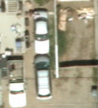 |
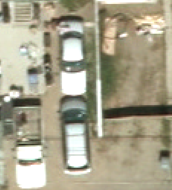 |
| Original | After JPEG/YCBCR |
|---|
Can you see the difference? Me neither. Using the default JPEG “quality” level of 75%, there are no visible artefacts. In general, JPEG is very good at compressing things so humans “can’t see” the lost information. I’d never use it for compressing a DEM or a data raster, but for a visual image, I use JPEG with impunity, and with much lower quality settings too (for more space saved).
What about a quality level of 50%?
gdal_translate \
  -b 1 -b 2 -b 3 \
  -co COMPRESS=JPEG \
  -co JPEG_QUALITY=50 \
  -co PHOTOMETRIC=YCBCR \
  -co TILED=YES \
  5255C.tif 5255C_JPEG_YCBCR_50.tif
See the quality difference? Possibly in the gravel road at the top, but it’s hard to say. In general on larger areas with very subtley changing colors you might get some visible compression artefacts.
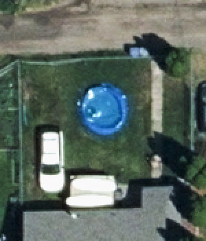 |
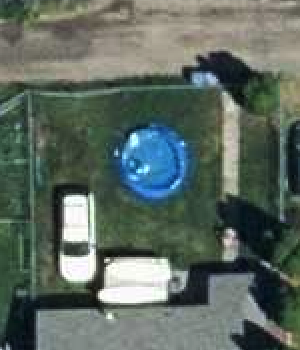 |
| Original | JPEG/YCBCR @ 50% |
|---|
And we dropped another 30% in file size! We are now less than 3% of the original file size.
5255C_JPEG_YCBCR_50.tif [18M]
Finally, for high speed serving at more zoomed out scales, we need to add overviews to the image. We’ll make sure the overviews use the same, high compression options as the base data.
gdaladdo \
  --config COMPRESS_OVERVIEW JPEG \
  --config JPEG_QUALITY_OVERVIEW 50 \
  --config PHOTOMETRIC_OVERVIEW YCBCR \
  --config INTERLEAVE_OVERVIEW PIXEL \
  -r average \
  5255C_JPEG_YCBCR_50.tif \
  2 4 8 16
For reasons passing understanding, gdaladdo uses a different set of command-line switches to pass the configuration info to the compressor than gdal_translate does, but as before, mine is not to reason why.
The final size, now with overviews as well as the original data, is still less that 1/25 the size of the original.
5255C_JPEG_YCBCR_50.tif [26M]
So, to sum up, your best format for image serving is:
- GeoTiff, so you can avoid proprietary image formats and nonsense, with
- JPEG compression, for visually fine results with much space savings, and
- (optionally) a more agressive JPEG quality setting, and
- YCBCR color, for even smaller size, and
- internal tiling, for fast access of random squares of data, and
- overviews, for fast access of zoomed out views of the data.
Go forth and compress!
What about COG?
Wait, I haven’t mentioned the new kid in imagery serving, the “cloud optimized GeoTIFF”! Maybe that is the answer now and all this stuff is moot?
As always in software, the answer is “it depends”. If you are storing your images online, in a cloud “object store” like AWS S3, or Azure Blob Storage, or Google Cloud Storage, or Cloudfare R2, then using COG as your format makes a lot of sense. The number of native COG clients is growing and COG clients can access the files directly in the cloud storage without downloading, which can be immensely useful.
To generate COG files with GDAL, use the new COG driver instead of the GeoTIFF driver. An equivalent GDAL COG-generating command to the final conversion in this post looks like this:
gdal_translate \
  -of COG \
  -co COMPRESS=JPEG \
  -co QUALITY=50 \
  5255C.tif 5255C_COG.tif
All the fancy stuff from above about tiling and overviews and YCBCR photometric spaces is automatically included in the GDAL COG output driver, so the command is a lot simpler.
5255C_COG.tif [25M]
And the output is still very efficiently compressed!
The COG file has all the same features as the basic GeoTIFF (efficient JPEG, tiling, overviews) and it has some extra metadata to make it easier and faster for native COG clients to read data from it, so there’s no reason not to always use the COG option, if your version of GDAL supports it.