


Parallel PostGIS II
31 Oct 2017A year and a half ago, with the release of PostgreSQL 9.6 on the horizon, I evaluated the parallel query infrastructure and how well PostGIS worked with it.
The results at the time were mixed: parallel query worked, when poked just the right way, with the correct parameters set on the PostGIS functions, and on the PostgreSQL back-end. However, under default settings, parallel queries did not materialize. Not for scans, not for joins, not for aggregates.
With the recent release of PostgreSQL 10, another generation of improvement has been added to parallel query processing, so it’s fair to ask, “how well does PostGIS parallelize now?”
TL;DR:
The answer is, better than before:
- Parallel aggregations now work out-of-the-box and parallelize in reasonable real-world conditions.
- Parallel scans still require higher function costs to come into action, even in reasonable cases.
- Parallel joins on spatial conditions still seem to have poor planning, requiring a good deal of manual poking to get parallel plans.
Setup
In order to run these tests yourself, you will need:
- PostgreSQL 10
- PostGIS 2.4
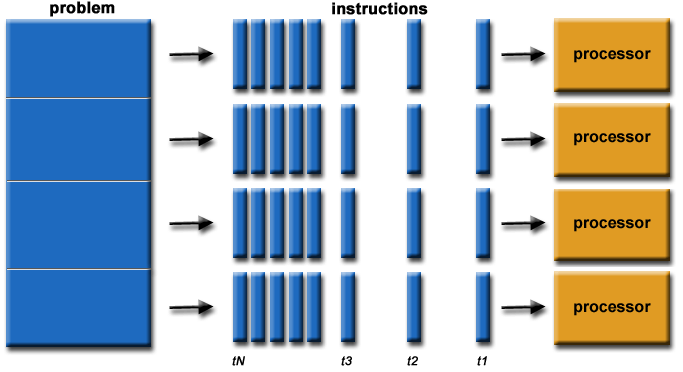
You’ll also need a multi-core computer to see actual performance changes. I used a 4-core desktop for my tests, so I could expect 4x improvements at best.
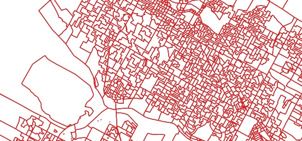
For testing, I used the same ~70K Canadian polling division polygons as last time.
createdb parallel
psql -c 'create extension postgis' parallel
shp2pgsql -s 3347 -I -D -W latin1 PD_A.shp pd | psql parallel
To support join queries, and on larger tables, I built a set of point tables based on the polling divisions. One point per polygon:
CREATE TABLE pts AS
SELECT
  ST_PointOnSurface(geom)::Geometry(point, 3347) AS geom,
  gid, fed_num
FROM pd;

CREATE INDEX pts_gix
  ON pts USING GIST (geom);
Ten points per polygon (for about 700K points):
CREATE TABLE pts_10 AS
SELECT
  (ST_Dump(ST_GeneratePoints(geom, 10))).geom::Geometry(point, 3347) AS geom,
  gid, fed_num
FROM pd;

CREATE INDEX pts_10_gix
  ON pts_10 USING GIST (geom);
One hundred points per polygon (for about 7M points):
CREATE TABLE pts_100 AS
SELECT
  (ST_Dump(ST_GeneratePoints(geom, 100))).geom::Geometry(point, 3347) AS geom,
  gid, fed_num
FROM pd;

CREATE INDEX pts_100_gix
  ON pts_100 USING GIST (geom);
The configuration parameters for parallel query have changed since the last test, and are (in my opinion) a lot easier to understand.
These parameters are used to fine-tune the planner and execution. Usually you don’t need to change them.
parallel_setup_costsets the planner’s estimate of the cost of launching parallel worker processes. Default 1000.parallel_tuple_costsets the planner’s estimate of the cost of transferring one tuple from a parallel worker process to another process. Default 0.1.min_parallel_table_scan_sizesets the minimum amount of table data that must be scanned in order for a parallel scan to be considered. Default 8MB.min_parallel_index_scan_sizesets the minimum amount of index data that must be scanned in order for a parallel scan to be considered. Default 512kB.force_parallel_modeforces the planner to parallelize is wanted. Values: off | on | regresseffective_io_concurrencyfor some platforms and hardware setups allows true concurrent read. Values from 1 (for one spinning disk) to ~100 (for an SSD drive). Default 1.
These parameters control how many parallel processes are launched for a query.
max_worker_processessets the maximum number of background processes that the system can support. Default 8.max_parallel_workerssets the maximum number of workers that the system can support for parallel queries. Default 8.max_parallel_workers_per_gathersets the maximum number of workers that can be started by a single Gather or Gather Merge node. Setting this value to 0 disables parallel query execution. Default 2.
Once you get to the point where #processes == #cores there’s not a lot of advantage in adding more processes. However, each process does exact a cost in terms of memory: a worker process consumes work_mem the same as any other backend, so when planning memory usage take both max_connections and max_worker_processes into consideration.
Before running tests, make sure you have a handle on what your parameters are set to: I frequently found I accidentally tested with max_parallel_workers set to 1.
show max_worker_processes;
show max_parallel_workers;
show max_parallel_workers_per_gather;
Aggregates
First, set max_parallel_workers and max_parallel_workers_per_gather to 8, so that the planner has as much room as it wants to parallelize the workload.
PostGIS only has one true spatial aggregate, the ST_MemUnion function, which is comically inefficient due to lack of input ordering. However, it’s possible to see some aggregate parallelism in action by wrapping a spatial function in a parallelizable aggregate, like Sum():
SET max_parallel_workers = 8;
SET max_parallel_workers_per_gather = 8;

EXPLAIN ANALYZE
  SELECT Sum(ST_Area(geom))
    FROM pd
Boom! We get a 3-worker parallel plan and execution about 3x faster than the sequential plan.
Finalize Aggregate
(cost=15417.45..15417.46 rows=1 width=8)
(actual time=236.925..236.925 rows=1 loops=1)
->  Gather
(cost=15417.13..15417.44 rows=3 width=8)
(actual time=236.915..236.921 rows=4 loops=1)
   Workers Planned: 3
   Workers Launched: 3
   ->  Partial Aggregate
   (cost=14417.13..14417.14 rows=1 width=8)
   (actual time=231.724..231.724 rows=1 loops=4)
       ->  Parallel Seq Scan on pd
       (cost=0.00..13800.30 rows=22430 width=2308)
       (actual time=0.049..30.407 rows=17384 loops=4)
Planning time: 0.111 ms
Execution time: 238.785 ms
Just to confirm, re-run it with parallelism turned off:
SET max_parallel_workers_per_gather = 0;

EXPLAIN ANALYZE
  SELECT Sum(ST_Area(geom))
    FROM pd
Back to one thread and taking about 3 times as long, as expected.
Scans
The simplest spatial parallel scan adds a spatial function to the filter clause.
SET max_parallel_workers = 8;
SET max_parallel_workers_per_gather = 8;

EXPLAIN ANALYZE
  SELECT *
    FROM pd
    WHERE ST_Area(geom) > 10000;
Unfortunately, that does not give us a parallel plan.
The ST_Area() function is defined with a COST of 10. If we move it up, to 100, we can get a parallel plan.
SET max_parallel_workers_per_gather = 8;

ALTER FUNCTION ST_Area(geometry) COST 100;
EXPLAIN ANALYZE
  SELECT *
    FROM pd
    WHERE ST_Area(geom) > 10000;
Boom! Parallel scan with three workers:
Gather
(cost=1000.00..20544.33 rows=23178 width=2554)
(actual time=0.253..293.016 rows=62158 loops=1)
Workers Planned: 5
Workers Launched: 5
->  Parallel Seq Scan on pd
    (cost=0.00..17226.53 rows=4636 width=2554)
    (actual time=0.091..210.581 rows=10360 loops=6)
     Filter: (st_area(geom) > '10000'::double precision)
     Rows Removed by Filter: 1229
Planning time: 0.128 ms
Execution time: 302.600 ms
It appears our spatial function costs may still be too low in general to get good planning. And as we will see with joins, it’s possible the planner is still discounting function costs too much in deciding whether to go parallel or not.
Joins
Starting with a simple join of all the polygons to the 100 points-per-polygon table, we get:
SET max_parallel_workers_per_gather = 4;

EXPLAIN
 SELECT *
  FROM pd
  JOIN pts_100 pts
  ON ST_Intersects(pd.geom, pts.geom);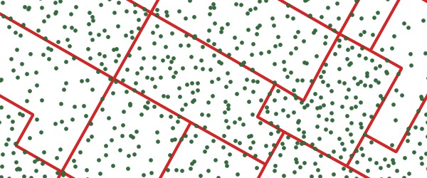
In order to give the PostgreSQL planner a fair chance, I started with the largest table, thinking that the planner would recognize that a “70K rows against 7M rows” join could use some parallel love, but no dice:
Nested Loop
(cost=0.41..13555950.61 rows=1718613817 width=2594)
 ->  Seq Scan on pd
     (cost=0.00..14271.34 rows=69534 width=2554)
 ->  Index Scan using pts_gix on pts
     (cost=0.41..192.43 rows=232 width=40)
       Index Cond: (pd.geom && geom)
       Filter: _st_intersects(pd.geom, geom)
There are a number of knobs we can press on. There are two global parameters:
parallel_setup_costdefaults to 1000, but no amount of lowering the value, even to zero, causes a parallel plan.parallel_tuple_costdefaults to 0.1. Reducing it by a factor of 100, to 0.001 causes the plan to flip over into a parallel plan.
SET parallel_tuple_cost = 0.001;As with all parallel plans, it is a nested loop, but that’s fine since all PostGIS joins are nested loops.
Gather  (cost=0.28..4315272.73 rows=1718613817 width=2594)
Workers Planned: 4
->  Nested Loop
    (cost=0.28..2596658.92 rows=286435636 width=2594)
     ->  Parallel Seq Scan on pts_100 pts
         (cost=0.00..69534.00 rows=1158900 width=40)
     ->  Index Scan using pd_geom_idx on pd
         (cost=0.28..2.16 rows=2 width=2554)
           Index Cond: (geom && pts.geom)
           Filter: _st_intersects(geom, pts.geom)
Running the parallel plan to completion on the 700K point table takes 18s with four workers and 53s with a sequential plan. We are not getting an optimal speed up from parallel processing anymore: four workers are completing in 1/3 of the time instead of 1/4.
If we set parallel_setup_cost and parallel_tuple_cost back to their defaults, we can also change the plan by fiddling with the function costs.
First, note that our query can be re-written like this, to expose the components of the spatial join:
SET parallel_tuple_cost=0.1;
SET parallel_setup_cost=1000;
SET max_parallel_workers_per_gather = 4;

EXPLAIN
 SELECT *
  FROM pd
  JOIN pts_100 pts
   ON pd.geom && pts.geom
   AND _ST_Intersects(pd.geom, pts.geom);
The default cost of _ST_Intersects() is 100. If we adjust it up by a factor of 100, we can get a parallel plan.
ALTER FUNCTION _ST_Intersects(geometry, geometry) COST 10000;However, what if our query only used a single spatial operator in the join filter? Can we still force a parallel plan on this query?
SET parallel_tuple_cost=0.1;
SET parallel_setup_cost=1000;
SET max_parallel_workers_per_gather = 4;

EXPLAIN
 SELECT *
  FROM pd
  JOIN pts_100 pts
  ON pd.geom && pts.geom;
The && operator could activate one of two functions:
geometry_overlaps(geom, geom)is bound to the&&operatorgeometry_gist_consistent_2d(internal, geometry, int4)is bound to the 2d spatial index
However, no amount of increasing their COST causes the operator-only query plan to flip into a parallel mode:
ALTER FUNCTION  geometry_overlaps(geometry, geometry) COST 1000000000000;
ALTER FUNCTION  geometry_gist_consistent_2d(internal, geometry, int4) COST 10000000000000;
So for operator-only queries, it seems the only way to force a spatial join is to muck with the parallel_tuple_cost parameter.
More Joins
Can we parallelize a common GIS use case: the spatial overlay?
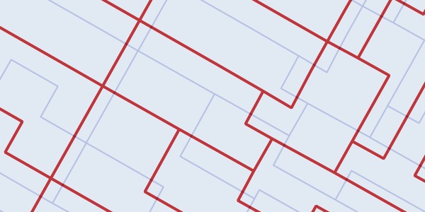
Here is a table that simply shifts the polling divisions up and over, so that they can be overlaid to create a new set of smaller polygons.
CREATE TABLE pd_translate AS
SELECT ST_Translate(geom, 100, 100) AS geom,
    fed_num, pd_num
  FROM pd;

CREATE INDEX pd_translate_gix
  ON pd_translate USING GIST (geom);
CREATE INDEX pd_fed_num_x
  ON pd (fed_num);
CREATE INDEX pdt_fed_num_x
  ON pd_translate (fed_num);
The overlay operation finds, for each geometry on one side, all the overlapping geometries, and then calculates the shape of those overlaps (the “intersection” of the pair). Calculating intersections is expensive, so it’s something want to happen in parallel, even more than we want the join to happen in parallel.
This query calculates the overlay of all polling divisions (and their translations) in British Columbia (fed_num > 59000):
EXPLAIN
SELECT ST_Intersection(pd.geom, pdt.geom) AS geom
  FROM pd
  JOIN pd_translate pdt
  ON ST_Intersects(pd.geom, pdt.geom)
  WHERE pd.fed_num > 59000
  AND pdt.fed_num > 59000;
Unfortunately, the default remains a non-parallel plan. The parallel_tuple_cost has to be adjusted down to 0.01 or the cost of _ST_Intersects() adjusted upwards to get a parallel plan.
Conclusions
- The costs assigned to PostGIS functions still do not provide the planner a good enough guide to determine when to invoke parallelism. Costs assigned currently vary widely without any coherent reasons.
- The planner behaviour on spatial joins remains hard to predict: is the deciding factor the join operator cost, the number of rows of resultants, or something else altogether? Counter-intuitively, it was easier to get join behaviour from a relatively small 6K x 6K polygon/polygon overlay join than it was for the 70K x 7M point/polygon overlay.