In my earlier post on new parallel query support coming in PostgreSQL 9.6 I was unable to come up with a parallel join query, despite much kicking and thumping the configuration and query.
It turns out, I didn’t have all the components of my query marked as PARALLEL SAFE, which is required for the planner to attempt a parallel plan. My query was this:
And _ST_Intersects() was marked as safe, but I neglected to mark the function behind the && operator – geometry_overlaps – as safe. With both functions marked as safe, and assigned a hefty function cost of 1000, I get this query:
 Nested Loop
 (cost=0.28..1264886.46 rows=21097041 width=2552)
 (actual time=0.119..13876.668 rows=69534 loops=1)
   ->  Seq Scan on pd
   (cost=0.00..14271.34 rows=69534 width=2512)
   (actual time=0.018..89.653 rows=69534 loops=1)
   ->  Index Scan using pts_gix on pts
   (cost=0.28..17.97 rows=2 width=40)
   (actual time=0.147..0.190 rows=1 loops=69534)
         Index Cond: (pd.geom && geom)
         Filter: _st_intersects(pd.geom, geom)
         Rows Removed by Filter: 2
 Planning time: 8.365 ms
 Execution time: 13885.837 ms
Hey wait! That’s not parallel either!
It turns out that parallel query involves a secret configuration sauce, just like parallel sequence scan and parellel aggregate, and naturally it’s different from the other modes (gah!)
The default parallel_tuple_cost is 0.1. If we reduce that by an order of magnitude, to 0.01, we get this plan instead:
 Gather
 (cost=1000.28..629194.94 rows=21097041 width=2552)
 (actual time=0.950..6931.224 rows=69534 loops=1)
   Number of Workers: 3
   ->  Nested Loop
   (cost=0.28..628194.94 rows=21097041 width=2552)
   (actual time=0.303..6675.184 rows=17384 loops=4)
         ->  Parallel Seq Scan on pd
         (cost=0.00..13800.30 rows=22430 width=2512)
         (actual time=0.045..46.769 rows=17384 loops=4)
         ->  Index Scan using pts_gix on pts
         (cost=0.28..17.97 rows=2 width=40)
         (actual time=0.285..0.366 rows=1 loops=69534)
               Index Cond: (pd.geom && geom)
               Filter: _st_intersects(pd.geom, geom)
               Rows Removed by Filter: 2
 Planning time: 8.469 ms
 Execution time: 6945.400 ms
Ta da! A parallel plan, and executing almost twice as fast, just like the doctor ordered.
Complaints
Mostly the parallel support in core “just works” as advertised. PostGIS does need to mark our functions as quite costly, but that’s reasonable since they actually are quite costly. What is not good is the need to tweak the configuration once the functions are properly costed:
Having to cut parallel_tuple_cost by a factor of 10 for the join case is not any good. No amount of COST increases seemed to have an effect, only changing the core parameter did.
Having to increase the cost of functions used in aggregates by a factor of 100 over cost of functions used in sequence filters is also not any good.
So, with a few more changes to PostGIS, we are quite close, but the planner for parallel cases needs to make more rational use of function costs before we have achieved parallel processing nirvana for PostGIS.
Parallel query support in PostgreSQL in the upcoming 9.6 release will be available for a number of query types: sequence scans, aggregates and joins. Because PostGIS tends to involve CPU-intensive calculations on geometries, support for parallel query has been at the top of our request list to the core team for a long time. Now that it is finally arriving the question is: does it really help?
TL;DR:
With some adjustments to function COST both parallel sequence scan and parallel aggregation deliver very good parallel performance results.
The cost adjustments for sequence scan and aggregate scan are not consistent in magnitude.
Parallel join does not seem to work for PostGIS indexes yet, but perhaps there is some magic to learn from PostgreSQL core on that.
Setup
In order to run these tests yourself, you will need to check out and build:
It’s worth noting that this data set is, in terms of number of rows very very small as databases go. This will become important as we explore the behaviour of the parallel processing, because the assumptions of the PostgreSQL developers about what constitutes a “parallelizable load” might not match our assumptions in the GIS world.
With the data loaded, we can do some tests on parallel query. Note that there are some new configuration options for parallel behaviour that will be useful during testing:
max_parallel_degree sets the maximum degree of parallelism for an individual parallel operation. Default 0.
parallel_tuple_cost sets the planner’s estimate of the cost of transferring a tuple from a parallel worker process to another process. The default is 0.1.
parallel_setup_cost sets the planner’s estimate of the cost of launching parallel worker processes. The default is 1000.
force_parallel_mode allows the use of parallel queries for testing purposes even in cases where no performance benefit is expected. Default ‘off’.
Parallel Sequence Scan
Before we can test parallelism, we need to turn it on! The default max_parallel_degree is zero, so we need a non-zero value. For my tests, I’m using a 2-core laptop, so:
SETmax_parallel_degree=2;
Now we are ready to run a query with a spatial filter. Using EXPLAIN ANALYZE suppressed the actual answer in favour of returning the query plan and the observed execution time:
 Aggregate
 (cost=14676.95..14676.97 rows=1 width=8)
 (actual time=757.489..757.489 rows=1 loops=1)
   ->  Seq Scan on pd
   (cost=0.00..14619.01 rows=23178 width=0)
   (actual time=0.160..747.161 rows=62158 loops=1)
         Filter: (st_area(geom) > 10000)
         Rows Removed by Filter: 7376
 Planning time: 0.137 ms
 Execution time: 757.553 ms
Two things we can learn here:
There is no parallelism going on here, the query plan is just a single-threaded one.
The single-threaded execution time is about 750ms.
Now we have a number of options to fix this problem:
We can force parallelism using force_parallel_mode, or
We can force parallelism by decreasing the parallel_setup_cost, or
We can adjust the cost of ST_Area() to try and get the planner to do the right thing automatically.
It turns out that the current definition of ST_Area() has a default COST setting, so it is considered to be no more or less expensive than something like addition or substraction. Since calculating area involves multiple floating point operations per polygon segment, that’s a stupid cost.
In general, all PostGIS functions are going to have to be reviewed and costed to work better with parallelism.
If we redefine ST_Area() with a big juicy cost, things might get better.
Some of the execution results output are wrong! They say that only 1844 rows were removed by the filter, but in fact 7376 were (as we can confirm by running the queries without the EXPLAIN ANALYZE). This is a known limitation, reporting on the results of only one parallel worker, which (should) maybe, hopefully be fixed before 9.6 comes out.
The execution time has been halved, just as we would hope for a 2-core machine!
Now for the disappointing part, try this:
EXPLAINANALYZESELECTST_Area(geom)FROMpd;
Even though the work being carried out (run ST_Area() on 70K polygons) is exactly the same as in our first example, the planner does not parallelize it, because the work is not in the filter.
 Seq Scan on pd
 (cost=0.00..31654.84 rows=69534 width=8)
 (actual time=0.130..722.286 rows=69534 loops=1)
 Planning time: 0.078 ms
 Execution time: 727.344 ms
For geospatial folks, who tend to do a fair amount of expensive calculation in the SELECT parameters, this is a bit disappointing. However, we still get impressive parallelism on the filter!
Parallel Aggregation
The aggregate most PostGIS users would like to see parallelized is ST_Union() so it’s worth explaining why that’s actually a little hard.
PostgreSQL Aggregates
All aggregate functions in PostgreSQL consist of at least two functions:
A “transfer function” that takes in a value and a transfer state, and adds the value to the state. For example, the Avg() aggregate has a transfer state consisting of the sum of all values seen so far, and the count of all values processed.
A “final function” that takes in a transfer state and converts it to the final aggregate output value. For example, the Avg() aggregate final function divides the sum of all values by the count of all values and returns that number.
For parallel processing, PostgreSQL adds a third kind of function:
A “combine” function, that takes in two transfer states and outputs a singe combined state. For the Avg() aggregate, this would add the sums from each state and counts from each state and return that as the new combined state.
So, in order to get parallel processing in an aggregate, we need to define “combine functions” for all the aggregates we want parallelized. That way the master process can take the completed transfer states of all parallel workers, combine them, and then hand that final state to the final function for output.
To sum up, in parallel aggregation:
Each worker runs “transfer functions” on the records it is responsible for, generating a partial “transfer state”.
The master takes all those partial “transfer states” and “combines” them into a “final state”.
The master then runs the “final function” on the “final state” to get the completed aggregate.
Note where the work occurs: the workers only run the transfer functions, and the master runs both the combine and final functions.
PostGIS ST_Union Aggregate
One of the things we are proud of in PostGIS is the performance of our ST_Union() implementation, which gains performance from the use of a cascaded union algorithm.
Cascaded union involves the following steps:
Collects all the geometries of interest into an array (aggregate transfer function), then
Builds a tree on those geometries and unions them from the leaves of the tree upwards (aggregate final function).
Note that all the hard work happens in the final step. The transfer functions (which is what would be run on the workers) do very little work, just gathering geometries into an array.
Converting this process into a parallel one by adding a combine function that does the union would not make things any faster, because the combine step also happens on the master. What we need is an approach that does more work during the transfer function step.
PostGIS ST_MemUnion Aggregate
“Fortunately” we have such an aggregate, the old union implementation from before we added “cascaded union”. The “memory friendly” union saves memory by not building up the array of geometries in memory, at the cost of spending lots of CPU unioning each input geometry into the transfer state.
In that respect, it is the perfect example to use for testing parallel aggregate.
The non-parallel definition of ST_MemUnion() is this:
No special types or functions required: the transfer state is a geometry, and as each new value comes in the two-parameter version of the ST_Union() function is called to union it onto the state. There is no final function because the transfer state is the output value. Making the parallel version is as simple as adding a combine function that also uses ST_Union() to merge the partial states:
 Aggregate
 (cost=14445.67..14445.93 rows=1 width=8)
 (actual time=2031.230..2031.231 rows=1 loops=1)
   ->  Seq Scan on pd
   (cost=0.00..14445.17 rows=199 width=2311)
   (actual time=0.124..66.835 rows=169 loops=1)
         Filter: (fed_num = 47005)
         Rows Removed by Filter: 69365
 Planning time: 0.278 ms
 Execution time: 2031.887 ms
The open question is, “can we combine the subtlety of the cascaded union algorithm with the brute force of parallel execution”?
Maybe, but it seems to involve magic numbers: if the transfer function paused every N rows (magic number) and used cascaded union to combine the geometries received thus far, it could possibly milk performance from both smart evaluation and multiple CPUs. The use of a magic number is concerning however, and the approach would be very sensitive to the order in which rows arrived at the transfer functions.
Parallel Join
To test parallel join, we’ll build a synthetic set of points, such that each point falls into one polling division polygon:
But the query plan has no parallel elements! Uh oh!
Aggregate
(cost=222468.56..222468.57 rows=1 width=8)
(actual time=13830.361..13830.362 rows=1 loops=1)
   ->  Nested Loop
   (cost=0.28..169725.95 rows=21097041 width=0)
   (actual time=0.703..13815.008 rows=69534 loops=1)
         ->  Seq Scan on pd
         (cost=0.00..14271.34 rows=69534 width=2311)
         (actual time=0.086..90.498 rows=69534 loops=1)
         ->  Index Scan using pts_gix on pts
         (cost=0.28..2.22 rows=2 width=32)
         (actual time=0.146..0.189 rows=1 loops=69534)
               Index Cond: (pd.geom && geom)
               Filter: _st_intersects(pd.geom, geom)
               Rows Removed by Filter: 2
 Planning time: 6.348 ms
 Execution time: 13843.946 ms
The plan does involve a nested loop, so there should be an opportunity for parallel join to work magic. Unfortunately no variation of the query or the parallel configuration variables, or the function costs will change the situation: the query refuses to parallelize!
The ST_Intersects() function is actually a SQL wrapper on top of the && operator and the _ST_Intersects() function, but unwrapping it and using the components directly also has no effect.
Unfortunately without the index operator the query is so inefficient it doesn’t matter that it’s being run in parallel, it will take days to run to completion.
 Gather
 (cost=1000.00..721919734.88 rows=1611658891 width=2552)
   Number of Workers: 2
   ->  Nested Loop
   (cost=0.00..576869434.69 rows=1611658891 width=2552)
         Join Filter: _st_intersects(pd.geom, pts.geom)
         ->  Parallel Seq Scan on pd
         (cost=0.00..13865.73 rows=28972 width=2512)
         ->  Seq Scan on pts
         (cost=0.00..1275.34 rows=69534 width=40)
So, thus far, parallel query seems to be a wet squib for PostGIS, though I hope with some help from PostgreSQL core we can figure out where the problem lies.
UPDATE: Marking the geometry_overlaps function which is bound to the && operator as PARALLEL SAFE allows PostgreSQL to generate parallel join plans when the index is in place.
Conclusions
While it is tempting to think “yay, parallelism! all my queries will run $ncores times faster!” in fact parallelism still only applies in a limited number of cases:
When there is a sequence scan large (costly) enough to be worth parallelizing.
When there is an aggregate large (costly) enough to be worth parallelizing, and the aggregate function can actually parallize the work effectively.
(Theoretically) when there is a (nested loop) join large (costly) enough to be worth parallelizing.
Additionally there is still work to be done on PostGIS for optimal use of the parallel features we have available:
Every function is going to need a cost, and those costs may have to be quite high to signal to the planner that we are not garden variety computations.
Differences in COST adjustments for different modes need to be explored: why was a 10000 cost needed to kick the aggregation into action, while a 100 cost sufficed for sequence scan?
Aggregation functions that currently back-load work to the final function may have to be re-thought to do more work in the transfer stage.
Whatever issue is preventing our joins from parallelizing needs to be tracked down.
All that being said, the potential is to see a large number of queries get $ncores faster, so this promises to be the most important core development we’ve seen since the extension framework arrived back in PostgreSQL 9.1.
Though once considered benign to many, metadata found in government e-mail and server logs is beginning to generate interest from knowledgable freedom-of-information applicants who file requests for these logs spanning large time frames.
And Information Commissioner Elizabeth Denham knows my secret:
In fact, my Office recently issued an Order on this very issue, in which an applicant requested metadata from message tracking logs relating to email traffic for several government ministries and public sector agencies.
I can no longer deny the truth: I am Metadata Man
The Origin Story
I donned my suit back in July of 2013. It was an interesting time:
Elizabeth Denham had reported out on the FOI implications of the “ethnic outreach scandal” and included some interesting notes about the use and abuse of government e-mail.
A scandal in Ontario revolving around the deliberate deletion of e-mail records made me wonder about the persistance of log files as a kind of guarantee of data integrity.
Edward Snowden had revealed that the US government was gathering massive amounts of metadata about public citizens; we would later learn that the Canadian government also engages in this kind of surveilance (it still does).
I wondered if government had the same open attitude about its own metadata that it appeared to have for the general public’s metadata.
Thanks to IT centralization, every mail sent or received by government goes through a handful of SMTP servers. Looking at headers on mail I had received from government, I could see the servers were running Microsoft Exchange. And like other servers, Exchange automatically generates logs of every e-mail processed. So I asked:
Message tracking log files (files beginning with MSGTRK in %ExchangeInstallPath%TransportRoles\Logs\MessageTracking) from e7hub01.idir.bcgov, e7hub02.idir.bcgov, e7hub03.idir.bcgov, e7hub04.idir.bcgov, e7hub05.idir.bcgov, e7hub06.idir.bcgov, e7hub07.idir.bcgov, e7hub08.idir.bcgov, e7hub09.idir.bcgov.
Date range is January 1, 2013 to July 3, 2013.
The log files do not contain email contents, only metadata such as:
the sender email address
the recipient email address
the date and time the email transitted the server
the unique message number for the email
the subject line of the email (Microsoft Exchange only)
Mail server log files are not under the control of mail recipients and senders, they are under the control of central IT administrators. So while political staff can delete the mails they receive or the mails they send, they cannot delete the log entries that prove the emails existed in the first place.
Except for the subject line, which is easily stripped from the log file, there’s little in any particular log entry that could be considered unreleasable under FOI exceptions:
no cabinet confidences
no policy advice
no personal information
etc…
When each entry can be boiled to “John sent an e-mail to Jim on February 13, 2013”, it’s hard to see how any particular entry can be withheld. So I entertained the (naïve) hope that the whole corpus would be releasable post-haste.
Ha ha ha ha ha. Ha ha.
The First Battle
The government initially attempted to deny the request based on “Section 43” of the Act.
43 If the head of a public body asks, the commissioner may authorize the public body to disregard requests under section 5 or 29 that
(a) would unreasonably interfere with the operations of the public body because of the repetitious or systematic nature of the requests, or
(b) are frivolous or vexatious.
Section 43 is supposed to protect public bodies from harassment. For example, if I submitted thousands of requests in an attempt to bury the government in paperwork, the requests could be denied under Section 43.
The Ministry argued that they would have to manually review every line of the log files prior to release, and since the log files were 100’s of millions of lines long, obviously that was an undue burden, so, “go away, Metadata Man!”.
The size and detail in Ministry response were the first hint of just how uneven this field of battle was going to be.
The Ministry fielded real, live lawyers, whose full-time job is to argue FOI cases.
They took actual affidavits from staff and submitted them as evidence.
They cited relevant case law from both courts and previous FOI cases.
They double-spaced it all and neatly numbered every paragraph!
However, they also called me “frivolous or vexatious”, which was hurtful, so I felt duty bound to sit down and hammer out a response. I too double-spaced and numbered every paragraph.
In the end, the Adjudicator ignored most of the arguments made by both the Ministry and by me, and ruled that my request was neither “frivolous” nor “vexatious”, according to definitions clarified in prior FOI rulings.
And so I learned another useful lesson about the FOI appeals process: not only was I heavily out-gunned from a legal skills and resources perspective, but also the decision might in the end hinge on a some fact I knew nothing about in the first place.
The Second Battle
Having lost the first round, the Ministry fell back to more defensible territory: Section 22, “a public body must refuse to disclose personal information to an applicant if the disclosure would be an unreasonable invasion of a third party’s personal privacy”.
If Section 22 can be found to apply to records in the log file, then the Ministry can circle back around and point to the volume of data and say “sorry Metadata Man, there’s no way we can review all those records to remove the private bits”.
The trouble with that argument, from the Ministry’s point of view, is that any given record is completely anodyne: “John sent an e-mail to Jim on February 13, 2013”.
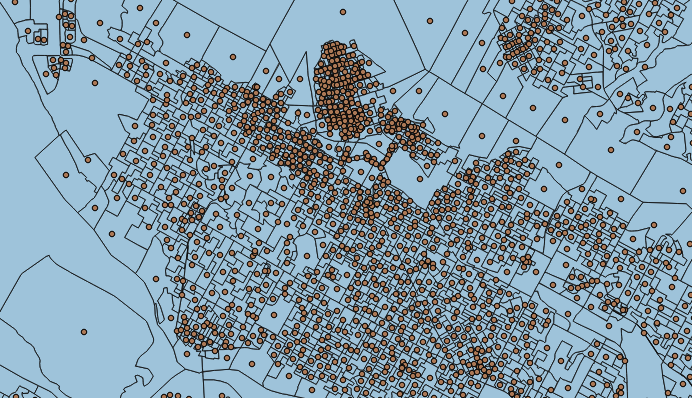
So they set about finding true examples of personal information in the data, by having BC Statistics run network analyses on the log files and comment on the network diagram.
From my review of the diagram, reporting structures are evident. In addition, relationships with individual outside the BC public service become evident. These may be business relationships or personal correspondance.
In my opinion, the graph also begins to hint at the sensitive information that might be revealed in this data set. In the lower centre, an individual has sent an email to “Fitness Centre”. There may be other accounts in government of a much more sensitive nature.
— Brad Williams Affidavit #1
To the staff in BC Stats who got to step out of the ordinary day-to-day grind and do network and relationship analyses to feed this process, depending on your level of intellectual curiousity: “you’re welcome”; or, “sorry”.
My case was getting harder to argue, but not impossible. There was definitely some provable personal information in the corpus, but the Ministry was still unable to point to any particular record and say “there! that is personal and private”. They were stuck hand-waving at potential “patterns of information” that might be there.
So my counter-argument acknowledged that while there might be some personal information in the data, the public interest in being able to monitor the actions of government (things like deleting important emails, and so on) out-weighed the private interest in keeping these thus-far-unproven data patterns private.
The message tracking logs are an important example of a government record, in that they are a huge corpus of data which should, because of their uncontroversial nature (from, to, date, id) be immediately releasable, but because of the possibility of personal information patterns, have become subject to this contentious process.
Imagine a document warehouse full of boxes of completely uncontroversial, releasable files. Imagine that the government refuses to release the files, because an employee at the warehouse may have placed his university transcript in one of the boxes. They are not sure he did so or not, but the effort of searching all the boxes is too high, therefore none of the boxes is releasable.
The situation with email logs is fundamentally the same. The question is not whether the effort of searching the boxes is too high: that’s a given, it’s too high. The question is whether the potential presence of a small piece of personal information is sufficient to block the release of a huge volume of public information.
— OIPC File F14-58135, Paul Ramsey, Mar 4, 2015
I liked my argument, it was simple and clear. But I also submitted my final argument with low expectations: the Information and Privacy Commissioner has always seemed to me to be an “information and PRIVACY Commissioner” in her priorities. In an OIPC decision balancing public access rights and privacy rights, the latter is more likely to win out.
the Ministry’s evidence demonstrates that the Logs reveal personal information, including information that is subject to a presumption that disclosure would be an unreasonable invasion of personal privacy. Against that, I recognize the valuable insights into the practical workings of government that could be gained from the applicant having access to the information.
However, this is insufficient to rebut the presumptions that apply to some of the information or to overcome the invasion of personal privacy that would result from disclosure of the Logs. Disclosure of some information in the requested information in the Logs would be an unreasonable invasion of personal privacy under s. 22.
— Hamish Flanagan, OIPC, Order F15-63
After over two years of process, my bulk request for the email server logs was at an end: Metadata Man was defeated.
Metadata Man Vindicated
However, within the ashes of defeat the seeds of a few victories could be found blooming.
The OIPC did not rule that all email log requests could be rejected, only those for which it was not possible to purge private information.
To be clear, my conclusion does not mean that metadata in the Logs can never be disclosed under FIPPA. The breadth of the applicant’s request means that the volume of responsive information allows patterns to be discerned that make disclosure in this particular case an unreasonable invasion of personal privacy. In a smaller subset of the same type of information, such patterns may not be so easily discerned so the personal privacy issues may be different.
— Hamish Flanagan, OIPC, Order F15-63
And the OIPC itself made use of email logs in investigating the illegal destruction of records in its report, “Access Denied”.
My investigators asked the Investigations and Forensics Unit to provide government’s message tracking logs for all of Duncan’s emails prior to November 21, 2014. My investigators then looked for terms in the subject lines of the emails such as “Highway of Tears” or “Highway 16”.
The query revealed six emails in his account predating his November 20, 2014 search
— OIPC Report F15-03, “Access Denied”
While denying the public the information access to carry out such research directly, the OIPC used the same technique to prepare one of its most politically explosive investigation reports.
The OIPC decision makes clear the technique needed to make a releasable request for message tracking logs:
Make the request small
Make the request targeted
So, if you think a particular employee is deleting the targets of your FOI requests, make simultaneous requests for the email itself and also for all message tracking log entries from and to the employee’s address.
For example, directed to the employee’s ministry:
All emails sent and received by jim.bob@gov.bc.ca between Jan 1 and Jan 8, 2017.
And directed to the Ministry of Citizen’s Services:
All e-mail message tracking log entries To: jim.bob@gov.bc.ca or From: jim.bob@gov.bc.ca between Jan 1 and Jan 8, 2017. Entries should include To, From, CC, Datetime, Message ID and Subject lines.
Even a very busy person is unlikely to generate more than a few dozen emails a day, so it is possible for FOI reviewers to manually scrub any private information from the log files. Similarly because the volume of records is low, there’s no leverage for pattern recognition algorithms to ascertain any information not visible in a line-by-line manual review.
For folks contemplating an FOI appeal, I have kept the full collection of documents submitted by myself and the Ministry during the process. Be prepared to spend a moderate amount of time reading and writing legalese.
Beyond the Borders of BC
The OIPC ruling should be of interest to information and privacy nerds in other parts of Canada and beyond because it provides real-world precedents of:
A government arguing forcefully that metadata is personal information.
A privacy commissioner ruling that metadata is personal information.
Against the backdrop of bulk harvesting of Canadian metadata by federal security agencies, and the same practice in the USA, having some institutional examples of governments arguing the opposite position might help in arguing for better behaviour at higher levels of government.
The BC government’s email retention policy (delete it all, whenever possible) was briefly back in the news last week as a BC Liberal staffer was brought up on charges:
George Steven Gretes has been charged with two counts of wilfully making false statements to mislead, or attempt to mislead, under the province’s Freedom of Information and Protection of Privacy Act. — CBC News
Sometimes, taking one for the team really means taking one for the team. But it’s important to remember that, however personally reprehensible Gretes’ actions were, his behaviour is just the tip of the ethical iceberg when it come to the current governments’ attitude towards record keeping.
It has been obvious for years that the government has a deliberate policy of poor management of digital records, and that there is a strong desire in high places to keep that policy in place. Gretes is not an isolated figure, he’s just the only person foolish and unlucky enough to be caught in deliberate law-breaking, instead of quietly taunting the public from the grey area.
Right in the middle of the exposure of Mr. Gretes’ actions last fall, the Opposition brought forward more evidence that political staffers routinely destroy records:
What we did last November is we asked for information pertaining to any e-mails from the chief of staff to the Minister of Natural Gas, Tobie Myers. Ms. Myers, of course, at the time we asked, was in discussions with people within the sector about legislation that was going to be before this House. What we got back from that request for information over a three-week period were three e-mails, just three.
It was curious to us that there would only be three e-mails in existence coming from the minister’s office over a three-week period, when flagship legislation was being tabled. So we asked for the message-tracking documents from the Minister of Citizens’ Services.
We determined through that route … that Ms. Myers sent 800 e-mails over that three-week period. So 797 triple deletes is a whole lot of triple deletes.
In those 800 e-mails, there were e-mails sent to Mr. Spencer Sproule, who may be familiar to members on this side. He used to work in the Premier’s office as her issue management director. He now, of course, is the chief spokesperson for Petronas, the lead agency looking at natural gas here in British Columbia.
Jared Kuehl, the head deputy of government relations at Shell; Neil Mackie, from AltaGas; and right to the minister’s office in Ottawa — 800 e-mails, and we got three.
My question is to the minister of openness and transparency in B.C. Liberal–land. Can he explain how it is that when we asked for 800, we only got three?
— John Horgan, Leader of the Opposition, Oct 26, 2015
The usual excuses are rolled out every time: the emails are “transitory” or they are filed “elsewhere”. Except these emails were from a high ranking Natural Gas ministry staffer to highly placed members of the industry! Transitory? Really? These were all just making plans to get coffee, 800 times?
The Information and Privacy Commissioner noted the same pattern in records keeping by the Premier’s Deputy Chief of Staff.
The Deputy Chief of Staff stated that her practice was to delete emails from her Sent Items folder on a daily basis and if all emails in that folder were of a transitory nature, she would delete all of them. Her evidence was that her Deleted Items folder was set to purge at the end of each day when she exited Microsoft Outlook.
— p50, Access Denied, OIPC, Oct 22, 2015
George Gretes must be quietly eating his liver, to be prosecuted for actions that he knows his former colleagues engage in every single day in their offices at the highest levels of government.
But that’s what it means to be the fall guy. The public thinks little of you because you were venal enough to do the crime. Your former friends think litle of you because you were stupid enough to get caught.
“It’s done. Now you don’t have to worry about it anymore.”
— George Gretes, on illegally deleting the target of an FOI request
Dealing with addresses is a common problem in information systems: people live and work in buildings which are addressed using “standard” postal systems. The trouble is, the postal address systems and the way people use them aren’t really all that standard.
Postal addressing systems are just standard enough that your average programmer can whip up a script to handle 80% of the cases correctly. Or a good programmer can handle 90%. Which just leaves all the rest of the cases. And also all the cases from countries where the programmer doesn’t live.
Counterexample: 8 Seven Gardens Burgh, WOODBRIDGE, IP13 6SU (pointed out by Raphael Mankin)
Most solutions to address parsing and normalization have used rules, hand-coded by programmers. These solutions can take years to write, as special cases are handled as they are uncovered, and are generally restricted in the language/country domains they cover.
There’s now an open source, empirical approach to address parsing and normalization: libpostal.
Libpostal is built using machine learning techniques on top of Open Street Map input data to produce parsed and normalized addresses from arbitrary input strings. It has binding for lots of languages: Perl, PHP, Python, Ruby and more.
And now, it also has a binding for PostgreSQL: pgsql-postal.
You can do the same things with the PostgreSQL binding as you can with the other languages: convert raw strings into normalized or parsed addresses. The normalization function returns an array of possible normalized forms:
SELECTunnest(postal_normalize('412 first ave, victoria, bc'));
                  unnest
------------------------------------------
 412 1st avenue victoria british columbia
 412 1st avenue victoria bc
(2 rows)
The parsing function returns a jsonb object holding the various parse components:
SELECTpostal_parse('412 first ave, victoria, bc');
The core library is very fast once it has been initialized, and the binding has been shown to be acceptably fast, despite some unfortunate implementation tradeoffs.
@pwramsey parsed and normalized 1.2 million rows in five minutes. *does happy dance*