16 Dec 2020
This post originally appeared on the Crunchy Data blog.
Summarizing data against a fixed grid is a common way of preparing data for analysis. Fixed grids have some advantages over natural and administrative boundaries:
- No appeal to higher authorities
- Equal unit areas
- Equal distances between cells
- Good for passing data from the “spatial” computational realm to a “non-spatial” realm
Ideally, we want to be able to generate grids that have some key features:
- Fixed origin point, so that grid can be re-generated and not move
- Fixed cell coordinates for a given cell size, so that the same cell can be referred to just using a cell address, without having to materialize the cell bounds
ST_SquareGrid()
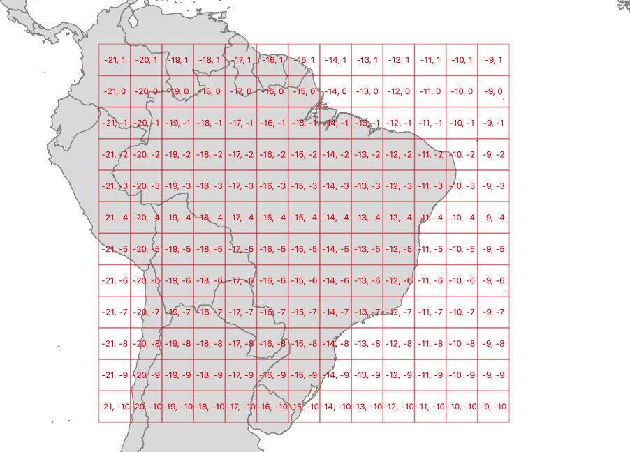
The ST_SquareGrid(size, bounds) function generates a grid with an origin at (0, 0) in the coordinate plane, and fills in the square bounds of the provided geometry.
SELECT (ST_SquareGrid(400000, ST_Transform(a.geom, 3857))).*
FROM admin a
WHERE name = 'Brazil';
So a grid generated using Brazil as the driving geometry looks like this.
ST_HexagonGrid()
The ST_HexagonGrid(size, bounds) function works much the same as the square grid function.
Hexagons are popular for some cartographic display purposes and modeling purposes. Surprisingly they can also be indexed using the same two-dimensional indexing scheme as squares.
The hexagon grid starts with a (0, 0) hexagon centered at the origin, and the gridding for a bounds includes all hexagons that touch the bounds.
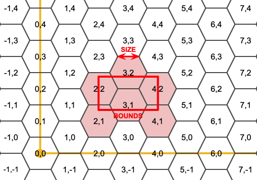
As with the square gridding, the coordinates of hexes are fixed for a particular gridding size.
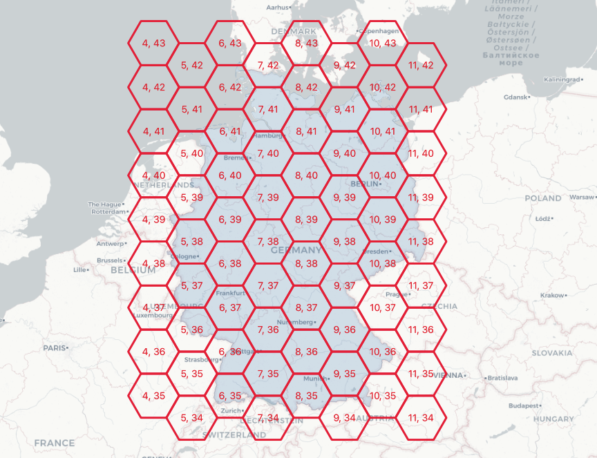
SELECT (ST_HexagonGrid(100000, ST_Transform(a.geom, 3857))).*
FROM admin a
WHERE name = 'Germany';
Here’s a 100km hexagon gridding of Germany.
Summarizing with Grids
It’s possible to materialize grid-based summaries, without actually materializing the grids, using the generator functions to create the desired grids on-the-fly.
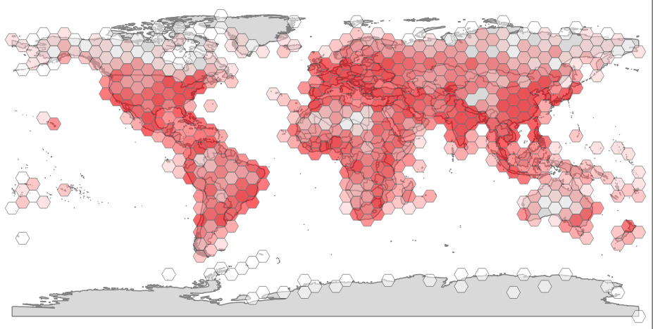
Here’s a summary of population points, using a hex grid.
SELECT sum(pop_max) as pop_max, hexes.geom
FROM
    ST_HexagonGrid(
        4.0,
        ST_SetSRID(ST_EstimatedExtent('places', 'geom'), 4326)
    ) AS hexes
    INNER JOIN
    places AS p
    ON ST_Intersects(p.geom, hexes.geom)
GROUP BY hexes.geom;
It’s also possible to join up on-the-fly gridding to visualization tools, for very dynamic user experiences, feeding these dynamically generated grids out to the end user via pg_tileserv.
16 Dec 2020
This post originally appeared on the Crunchy Data blog.
Open source developers sometimes have a hard time figuring out what feature to focus on, in order to generate the maximum value for end users. As a result, they will often default to performance.
Performance is the one feature that every user approves of. The software will keep on doing all the same cool stuff, only faster.
For PostGIS 3.1, there have been a number of performance improvements that, taken together, might add up to a substantial performance gain for your workloads.
Large Geometry Caching
Spatial joins have been slowed down by the overhead of large geometry access for a very long time.
SELECT A.*, B.*
FROM A
JOIN B
ON ST_Intersects(A.geom, B.geom)
PostgreSQL will plan and execute spatial joins like this using a “nested loop join”, which means iterating through one side of the join, and testing the join condition. This results in executions that look like:
- ST_Intersects(A.geom(1), B.geom(1))
- ST_Intersects(A.geom(1), B.geom(2))
- ST_Intersects(A.geom(1), B.geom(3))
So one side of the test repeats over and over.
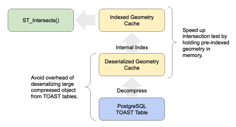
Caching that side and avoiding re-reading the large object for each iteration of the loop makes a huge difference to performance. We have seen 20 times speed-ups in common spatial join workloads (see below).
The fixes are quite technical, but if you are interested we have a detailed write-up available.
The on-disk format for geometry includes a short header that includes information about the geometry bounds, the spatial reference system and dimensionality. That means it’s possible for some functions to return an answer after only reading a few bytes of the header, rather than the whole object.
However, not every function that could do a fast read, did do a fast read. That is now fixed.
Faster Text Generation
It’s pretty common for web applications and others to generate text formats inside the database, and the code for doing so was not optimized. Generating “well-known text” (WKT), GeoJSON, and KML output all now use a faster path and avoid unnecessary copying.
PostGIS also now uses the same number-to-text code as PostgreSQL, which has been shown to be faster, and also allows us to expose a little more control over precision to end users.
How Much Faster?
For the specific use case of spatially joining, here is my favourite test case:
Load the data into both versions.
shp2pgsql -D -s 4326 -I ne_10m_admin_0_countries admin | psql postgis30
shp2pgsql -D -s 4326 -I ne_10m_populated_places places | psql postgis30
Run a spatial join that finds the sum of populated places in each country.
EXPLAIN ANALYZE
SELECT Sum(p.pop_max) as pop_max, a.name
FROM admin a
JOIN places p
ON ST_Intersects(a.geom, p.geom)
GROUP BY a.name
Average time over 5 runs:
- PostGIS 3.0 = 23.4s
- PostGIS 3.1 = 0.9s
This test is somewhat of a “worst case”, in that there are lots of very large countries in the admin data, but it gives an idea of the kind of speed-ups that are available for spatial joins against collections that include larger (250+ coordinates) geometries.
09 Dec 2020
Yesterday, Mapbox announced that they were moving their Mapbox GL JS library from a standard BSD license to a new very much non-open source license.
Joe Morrison said the news “shook” him (and also the readers of the Hacker News front page, well done Joe). It did me as well. Although apparently for completely different reasons.
Mapbox is the protagonist of a story I’ve told myself and others countless times. It’s a seductive tale about the incredible, counterintuitive concept of the “open core” business model for software companies.
– Joe Morrison
There’s a couple things wrong with Joe’s encomium to Mapbox and “open core”:
- first, Mapbox was never an open core business;
- second, open core is a pretty ugly model that has very little to do with the open source ethos of shared intellectual pursuit.

Mapbox was never Open Core
From the very start (well, at least from the early middle), Mapbox was built to be a location-based services business. It was to be the Google Maps for people who were unwilling to accept the downsides of Google Maps.
Google Maps will track you. They will take your data exhaust and ruthlessly monetize it. They will take your data and use it to build a better Google Maps that they will then re-sell to others.
If you value your data at all (if you are, say, a major auto maker), you probably don’t want to use Google Maps, because they are going to steal your data while providing you services. Also, Google Maps is increasingly the “only game in town” for location based services, and it seems reasonable to expect price increases (it has already happened once).

Nobody can compete with Google Maps, can they? Why yes, they can! Mapbox fuses the collaborative goodness of the OpenStreetMap community with clever software that enables the kinds of services that Google sells
(map tiles,
geocoding,
routing,
elevation services), and a bunch of services Google doesn’t sell (like custom map authoring) or won’t sell (like automotive vision).
But like Google, the value proposition Mapbox sells isn’t in the software, so much as the data and the platform underneath. Mapbox has built a unique, scalable platform for handling the huge problem of turning raw OSM data into usable services, and raw location streams into usable services. They sell access to that platform.
Mapbox has never been a software company, they’ve always been a data and services company.
The last company I worked for, CARTO, had a similar model, only moreso. All the parts of their value proposition (PostgreSQL, PostGIS, the CARTO UI, the tile server, the upload, everything) are open source. But they want you to pay them when you load your data into their service and use their software there. How can that be? Well, do you want to assemble all those open source parts into a working system and keep it running? Of course not. You just want to publish a map, or run an analysis, or add a spatial analysis to an existing system. So you pay them money.
Is Mapbox an “open core” company? No, is there a “Mapbox Community Edition” everyone can have, but an “Enterprise Edition” that is only available under a proprietary license? No. Does Mapbox even sell any software at all? No. (Yes, some.) They (mostly) sell services.
So what’s with the re-licensing? I’ll come back to that, but first…
Open Core is a Shitty Model
Actually, no, it seems to be a passable monetization model, for some businesses. It’s a shitty open source model though.
- MongoDB has an open source core, and sells a bunch of proprietary enterprise add-ons. They’ve grown very fast and might even reach sufficient velocity to escape their huge VC valuation (or they may yet be sucked into the singularity).
- Cloudera before them reached huge valuations selling proprietary add-ons around the open Hadoop ecosystem.
- MySQL flirted with an open core model for many years, but mostly stuck to spreading FUD about the GPL in order to get customers to pay them for proprietary licenses.
Easily the strangest part of the MySQL model was trash-talking the very open source license they chose to place their open source software under.
All those companies have been quite succesful along the axes of “getting users” and “making money”. Let me tell you why open core is nonetheless a shitty model:
- Tell me about the MongoDB developer community. Where do they work? Oh right, Mongo.
- Tell me about the Cloudary developer community? Where do they work?
- Tell me about the MySQL developer community? Where to they work? Oh right, Oracle. (There’s a whole other blog post to be written about why sole corporate control of open source projects is a bad idea.)
A good open source model is one that promotes heterogeneity of contributors, a sharing of control, and a rising of all boats when the software succeeds. Open core is all about centralizing gain and control to the sponsoring organization.
This is going to sound precious, but the leaders of open core companies don’t “care” about the ethos of open source. The CEOs of open core companies view open source (correctly, from their point of view) as a “sales channel”. It’s a way for customers to discover their paid offerings, it’s not an end in itself.

We didn’t open source it to get help from the community, to make the product better. We open sourced as a freemium strategy; to drive adoption.
– Dev Ittycheria, CEO, MongoDB
So, yeah, open core is a way to make money but it doesn’t “do” anything for open source as a shared proposition for building useful tools anyone can use, for anything they find useful, anytime and anywhere they like.
Check out Adam Jacob’s take on the current contradictions in the world of open source ethics; there are no hard and fast answers.
Mapbox Shook Me Too
I too was a little shook to learn of the Mapbox GL JS relicensing, but perhaps not “surprised”. This had happened before, with Tilemill (open) morphing into Mapbox Studio (closed).
The change says nothing about “open source” in the large as a model, and everything about “single vendor projects” and whether you should, strategically, believe their licensing.

I (and others) took the licensing (incorrectly) of Mapbox GL JS to be a promise, not only for now but the future, and made decisions based on that (incorrect) interpretation. I integrated GL JS into an open source project and now I have to revisit that decision.
The license change also says something about the business realities Mapbox is facing going forward. The business of selling location based services is a competitive one, and one that is perhaps not panning out as well as their venture capital valuation (billions?) would promise.
No doubt the board meetings are fraught. Managers are casting about for future sources of revenue, for places where more potential customers can be squeeeeezed into the sales funnel.
I had high hopes for Mapbox as a counterweight to Google Maps, a behemoth that seems likely to consume us all. The signs that the financial vice is beginning to close on it, that the promise might not be fulfilled, they shake me.
So, yeah, Joe, this is big news. Shaking news. But it has nothing to do with “open source as a business model”.
19 Nov 2020
This is a guest post from Raúl Marín, a core PostGIS contributor and a former colleague of mine at Carto. Raúl is an amazing systems engineer and has been cruising through the PostGIS code base making things faster and more efficient. You can find the original of this post at his new personal tech blog. – Paul
I’m not big on creating new things, I would rather work on improving something that’s already in use and has proven its usefulness. So whenever I’m thinking about what I should do next I tend to look for projects or features that are widely used, where the balance between development and runtime costs favors a more in depth approach.
Upon reviewing the changes of the upcoming PostGIS 3.1 release, it shouldn’t come as a surprise then that most of my contributions are focused on performance. When in doubt, just make it faster.
Since CARTO, the company that pays for my lunch, uses PostGIS’ Vector Tile functions as its backend for dynamic vector maps, any improvement there will have a clear impact on the platform. This is why since the appearance of the MVT functions in PostGIS 2.4 they’ve been enhanced in each major release, and 3.1 wasn’t going to be any different.
In this occasion the main reason behind the changes wasn’t the usual me looking for trouble, but the other way around. As ST_AsMVT makes it really easy to extract information from the database and into the browser, a common pitfall is to use SELECT * to extract all available columns which might move a lot of data unnecessarily and generate extremely big tiles. The easy solution to this problem is to only select the properties needed for the visualization but it’s hard to apply it retroactively once the application is in production and already depending on the inefficient design.
So there I was, looking into why the OOM killer was stopping databases, and discovering queries using a massive amount of resources to generate tiles 50-100 times bigger than they should (the recommendation is smaller than 500 KB). And in this case, the bad design of extracting all columns from the dataset was worsened by the fact that is was being applied to a large dataset; this triggered PostgreSQL parallelism requiring extra resources to generate chunks in parallel and later merge them together. In PostGIS 3.1 I introduced several changes to improve the performance of these 2 steps: the parallel processing and the merge of intermediate results.
The changes
Without getting into too much detail, the main benefit comes from changing the vector tile .proto such that a feature can only hold one value at a time. This is what the specification says, but not what the .proto enforces, therefore the internal library was allocating memory that it never used.
There are other additional changes, such as improving how values are merged between parallel workers, so feel free to have a look at the final commit itself if you want more details.
The best way to see the impact of these changes is through some examples. In both cases I am generating the same tile, in the same exact server and with the same dependencies; the only change was to replace the PostGIS library, which in 3.0 to 3.1 doesn’t require an upgrade.
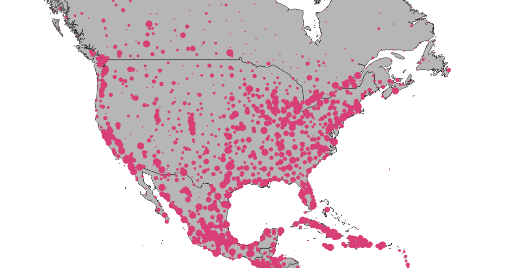
In the first example the tile contains all the columns of the 287k points in it. As I’ve mentioned before, it is discouraged to do this, but it is the simplest query to generate.

And for the second example, I’m generating the same tile but now only including the minimal columns for the visualization:

We can see, both in 3.0 and 3.1, that adding only the necessary properties makes things 10 times as fast as with the full data, and also that Postgis 3.1 is 30-40% faster in both situations.
Memory usage
Aside from speed, this change also greatly reduces the amount of memory used to generate a tile.
To see it in action, we monitor the PostgreSQL process while it’s generating the tile with all the properties. In 3.0, we observe in the blue line that the memory usage increases with time until it reaches around 2.7 GB at the end of the transaction.

We now monitor the same request on a server using Postgis 3.1. In this case the server uses around a third of the memory as in 3.0 (1GB vs 2.7GB) and, instead of having a linear increase, the memory is returned back to the system as soon as possible.
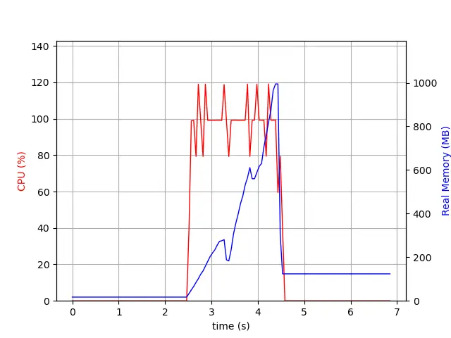
To sum it all up: PostGIS 3.1 is faster and uses less memory when generating large vector tiles.
15 Nov 2020
Way back in the 1980s, the Vander Zalm government privatized BC highways maintenance. They let out big contracts to private companies (fortunately this was before the era of international infrastructure firms, so they were local companies) and sold off the government road building machinery. The government employees union was naturally apoplectic and very much wanted the decision reversed. An NDP government took power at the next election, and… nothing changed.
The omlette was unscramblable. The expense and disruption of re-constituting the old highways maintenance department outweighed the cost. The machinery was all sold. The government had other fish to fry. It didn’t happen then. It hasn’t happened yet. Highways maintenance is still outsourced.
With that out of the way, here’s the latest data on BC information technology outsourcing.

The political economy of changing the trend was never good. On the side of change, was a line in the Minister of Citizens Services 2017 mandate letter:
Institute a cap on the value and the length of government IT contracts to save money, increase innovation, improve competition and help our technology sector grow.
On the side of more of the same, are:
- Existing relationships between civil servants and service providers.
- Contractual obligations that still have multiple years to run.
- Fear of change, including risk of service disruptions amidst big organizational changes.
- Comfort of stasis, just renew contracts and keep slowly growing budgets.
- Deep lack of political sexiness of internal IT issues.
- No one at the political level who is invested in the issue. (See previous.)
The UK IT reform experience, which is still ongoing in fits and starts, got off to a fast start because of the enthusiastic backing of the Cabinet Office Minister, Sir Francis Maude. It quickly hit the rocks after Maude retired and they lost his political cover.
Getting out from under these contracts is the right thing to do, but it’s the right thing to do in very abstract and theoretical ways:
- We want government to be more nimble and able to react to changes in society and policy.
- The machinery of government runs on information.
- The closer the people who work on the information are to the people working the policy, the easier it is for them to understand and react to their needs.
- Outsourced IT places a contractual buffer between the people who need the information services and the people who provide those services. It optimizes for the predictable and charges heavily for the novel.
There’s no easy big guaranteed win, and no press conference, and no glory. Just more reactive information services with incentives that align more closely to those of the people trying to deliver value to the people of BC. It’s technocratic, dull, worth doing, and probably not going to happen.
Anyways, back to the horse race.

The big surprise for me continues to be Maximus. Still billing strong, even with MSP premiums phased out? The MSP premium elimination date was January 1, 2020, so maybe this year will finally be the one we see a big drop in Maximus billings.
The continued growth of local companies is a positive trend. These aren’t Mom’n’Pop shops, I don’t track those, but companies with revenues north of several millions. Altogether they are still doing less business than IBM alone, but it’s a solid 10% of the total now.
It’s possible I’m being overly pessimistic. The biggest components of the IT outsourcing budget are the Telus and ESIT contracts, both of which end in 2021. But the easy thing is to just renew and move on, and in a world of Covid and recessions and many other issues much nearer to the daily lives of citizens I would not be surprised to see this issue languish.


