Here in the Covid-times, I haven’t been able to keep up my previous schedule of speaking at conferences, but I have managed to participate in a couple of episodes of the MapScaping Podcast, hosted by Daniel O’Donohue.
Spatial SQL - GIS without the GIS reviewed some history of SQL, the bestest data language in the wide, wide world, and how SQL fits into the world of geospatial software tools.
Daniel is a great interviewer and really puts together a tight show. So far I’ve been on two, and I quietly hope to join him again some time in the future.
Have you ever watched a team of five-year-olds play soccer? The way the mass of children chases the ball around in a group? I think programmers do that too.
There’s something about working on a problem together that is so much more rewarding than working separately, we cannot help but get drawn into other peoples problems. There’s a lot of gratification to be had in finding a solution to a shared difficulty!
Even better, different people bring different perspectives to a problem, and illuminate different areas of improvement.
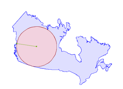
Maximum Inscribed Circle
A couple months ago, my colleague Martin Davis committed a pair of new routines into JTS, to calculate the largest circles that can fit inside a polygon or in a collection of geometries.
When I ported the GEOS test cases, I turned up some odd performance problems. The calculation seemed to be taking inordinately long for larger inputs. What was going on?
The “maximum inscribed circle” algorithm leans heavily on a routine called IndexedFacetDistance to calculate distances between polygon boundaries and candidate circle-centers while converging on the “maximum inscribed circle”. If that routine is slow, the whole algorithm will be slow.
Dan Baston, who originally ported the “IndexedFacetDistance” class got interested and started looking at some test cases of his own.
He found he could improve his old implementation using better memory management that he’d learned in the meantime. He also found some short-circuits to envelope distance calculation that improved performance quite a bit.
In fact, they improved performance so much that Martin ported them back to JTS, where he found that for some cases he could log a 10x performance in distance calculations.
There’s something alchemical about the whole thing.
There was a bunch of long-standing code nobody was looking at.
I ported an unrelated algorithm which exercised that code.
I wrote a test case and reported some profiling information.
Other folks with more knowledge were intrigued.
They fed their knowledge back and forth and developed more tests.
Improvements were found that made everything faster.
I did nothing except shine a light in a dark hole, and everyone else got very excited and things happened.
Toast Caching Redux
In a similar vein, as I described in my last diary entry, a long-standing performance issue in PostGIS was the repeated reading of large geometries during spatial joins.
Much of the problem was solved by dropping a very small “TOAST cache” into the process by which PostGIS reads geometries in functions frequently used in spatial joins.
I was so happy with the improvement the TOAST cache provided that I just stopped. Fortunately, my fellow PostGIS community member Raúl Marín was more stubborn.
The integrated system now uses TOAST identifiers to note identical repeated inputs and avoid both unneccessary reads off disk and unncessary cache checks of the index cache.
The result is that, for spatial joins over large objects, PostGIS 3.1 will be as much as 60x faster than the performance in PostGIS 3.0.
I prepared a demo for a bid proposal this week and found that an example query that took 800ms on my laptop took a full minute on the beefy 16-core demo server. What had I done wrong? Ah! My laptop is running the latest PostGIS code (which will become 3.1) while the cloud server was running PostGIS 2.4. Mystery solved!
Port, Port, Port
I may have mentioned that I’m not a very good programmer.
My current task is definitely exercising my imposter syndrome: porting Martin’s new overlay code from JTS to GEOS.
I knew it would take a long time, and I knew it would be a challenge; but knowing and experiencing are quite different things.
The challenges, as I’ve experienced them are:
Moving from Java’s garbage collected memory model to C++’s managed memory model means that I have to understand the object life-cycle which is implicit in Java and make it explicit in C++, all while avoiding accidentally introducing a lot of memory churn and data copying into the GEOS port. Porting isn’t a simple matter of transcribing and papering over syntactic idiom, it involves first understanding the actual JTS algorithms.
The age of the GEOS code base, and number of contributors over time, mean that there are a huge number of different patterns to potentially follow in trying to make a “consistent” port to GEOS. Porting isn’t a matter of blank-slate implementation of the JTS code – the ported GEOS code has to slot into the existing GEOS layout. So I have to spend a lot of time learning how previous implementations chose to handle life cycles and call patterns (pass reference, or pointer? yes. Return value? or void return and output parameter? also yes.)
My lack of C++ idiom means I spend an excessive amount of time looking up core functions and methods associated with them. This is the only place I’ve felt myself measurably get better over the past weeks.
I’m still only just getting started, having ported some core data structures, and little pieces of dependencies that the overlay needs. The reward will be a hugely improved overlay code for GEOS and thus PostGIS, but I anticipate the debugging stage of the port will take quite a while, even when the code is largely complete.
Wish me luck, I’m going to need it!
If you would like to test the new JTS overlay code, it resides on this branch. If you would like to watch me suffer as I work on the port, the GEOS branch is here.
I don’t plan well, I tend to hack first and try and find the structure afterwards. I am easily distracted. It takes me an exceedingly long time to marshal a problem in my head enough to attack it.
That said, the enforced slow-down from pandemic time has given me the opportunity to sit and look at code, knowing nothing else is coming down the pipe. There are no talks to prepare, no big-think keynotes to draft. I enjoy those things, and I really enjoy the ego-boost of giving them, but the preparation of them puts me in a mental state that is not conducive to doing code work.
So the end of travel has been good, for at least one aspect of my professional work.
The Successful Failure
Spatial operations against large objects have always been a performance hot spot.
The first problem is that large objects are … large. So if you have algorithms that scale O(n^2) on the number of vertices large objects will kill you. Guess what? Distance, intersects tests, and so on are all O(n^2) in their basic implementations.
We solved this problem a long time ago in PostGIS by putting in an extra layer of run-time indexing.
During a query (for those functions where it makes sense) if we see the same object twice in a row, we build an index on the edges of that object and keep the index in memory, for the life of the query. This gives us O(log(n)) performance for intersects, point-in-polygon, and so on. For joins in particular, this pattern of “seeing the same big thing multiple times” is very common.
This one small trick is one reason PostGIS is so much faster than “the leading brands”.
However, in order to “see the same object twice” we have to, for each function call in the query, retrieve the whole object, in order to compare it against the one we are holding in memory, to see if it is the same.
Here we run into an issue with our back-end.
PostgreSQL deals with large objects by (a) compressing them and (b) cutting the compressed object into slices and storing them in a side table. This all happens in the background, and is why you can store 1GB objects transparently in a database that has only an 8KB page size.
It’s quite computationally expensive, though. So much so that I found that simply bypassing the compression part of this feature could provide 5x performance gains on our spatial join workload.
At a code sprint in 2018, the PostGIS team agreed on the necessary steps to work around this long-standing performance issue.
Enhance PostgreSQL to allow partial decompression. This would allow the PostGIS caching system to retrieve just a little bit of large objects and use that part to determine if the object was not already in the cache.
Enhance the PostGIS serialization scheme to add a hashcode at the front of each large object. This way “is this a new object” could be answered with just a few bytes of hash, instead of checking the whole object.
Actually update the caching code code to use hash code and avoid unneccessary object retrievals.
Since this involved a change in PostgreSQL, which runs on an annual release cycle, and a change to the PostGIS serialization scheme, which is a major release marker, the schedule for this work was… long term.
Still, I managed to slowly chip away at it, goal in mind:
Last year I got compressed TOAST slicing added to PostgreSQL, which provided immediate performance benefits for some existing large object workloads.
That left adding the hash code to the front of the objects, and using that code in the PostGIS statement cache.
And this is where things fall apart.
The old statement cache was focussed on ensuring the in-memory indexes were in place. It didn’t kick in until the object had already been retrieved. So avoiding retrieval overhead was going to involve re-working the cache quite a bit, to handle both object and index caching.
I started on the work, which still lives on in this branch, but the many possible states of the cache (do I have part of an object? a whole object? an indexed object?) and the fact that it was used in multiple places by different indexing methods (geography tree, geometry tree, GEOS tree), made the change worrisomely complex.
And so I asked a question, that I should have asked years ago, to the pgsql-hackers list:
… within the context of a single SQL statement, will the Datum values for a particular object remain constant?
Basically, could I use the datum values as unique object keys without retrieving the whole object? That would neatly remove any need to retrieve full objects in order to determine if the cache needed to be updated. As usual, Tom Lane had the answer:
Jeez, no, not like that.
Oh, “good news”, I guess, my work is not in vain. Except wait, Tom included a codicil:
The case where this would actually be worth doing, probably, is where you are receiving a toasted-out-of-line datum. In that case you could legitimately use the toast pointer ID values (va_valueid + va_toastrelid) as a lookup key for a cache, as long as it had a lifespan of a statement or less.
Hm. So for a subset of objects, it was possible to generate a unique key without retrieving the whole object.
And that subset – “toasted-out-of-line datum” – were in fact the objects causing the hot spot: objects large enough to have been compressed and then stored in a side table in 8KB chunks.
What if, instead of re-writing my whole existing in-memory index cache, I left that in place, and just added a simple new cache that only worried about object retrieval. And only cached objects that it could obtain unique keys for, these “toasted-out-of-line” objects. Would that improve performance?
It did. By 20 times on my favourite spatial join benchmark. In increased it by 5 times on a join where only 10% of the objects were large ones. And on joins where none of the objects were large, the new code did not reduce performance at all.
And here’s the punch line: I’ve known about the large object hot spot for at least 5 years. Probably longer. I put off working on it because I thought the solution involved core changes to PostgreSQL and PostGIS, so first I had to put those changes in, which took a long time.
Once I started working on the “real problem”, I spent a solid week:
First on a branch to add hash codes, using the new serialization mechanisms from PostGIS 3.
Then on a unified caching system to replace the old in-memory index cache.
And then I threw all that work away, and in about 3 hours, wrote and tested the final patch that gave a 20x performance boost.
So, was this a success or a failure?
I’ve become inured to the huge mismatch in “time spent versus code produced”, particularly when debugging. Spending 8 hours stepping through a debugger to generate a one-line patch is pretty routine.
But something about the mismatch between my grandious and complex solution (partial retrieval! hash code!) and the final solution (just ask! try the half-measure! see if it’s better!) has really gotten on my nerves.
I like the win, but the path was a long and windy one, and PostGIS users have had slower queries than necessary for years because I failed to pose my simple question to the people who had an answer.
The Successful Success
Contra to that story of the past couple weeks, this week has been a raging success. I keep pinching myself and waiting for something to go wrong.
A number of years ago, JTS got an improvement to robustness in some operations by doing determinant calculations in higher precision than the default IEEE double precision.
Those changes didn’t make it into GEOS. There was an experimental branch, that Mateusz Loskot put together, and it sat un-merged for years, until I picked it up last fall, rebased it and merged it. I did so thinking that was the fastest way, and probably it was, but it included a dependency on a full-precision math library, ttmath, which I added to our tree.
Unfortunately, ttmath is basically unmaintained now.
And ttmath is arbitrary precision, while we really only need “higher precision”. JTS just uses a “double double” implementation, that uses the register space of two doubles for higher precision calculations.
And ttmath doesn’t support big-endian platforms (like Sparc, Power, and other chips), which was the real problem. We couldn’t go on into the future without support for these niche-but-not-uncommon platforms.
And ttmath includes some fancy assembly language that makes the build system more complex.
Fortunately, the JTS DD is really not that large, and it has no endian assumptions in it, so I ported it and tested it out against ttmath.
It’s smaller.
It’s faster. (About 5-10%. Yes, even though it uses no special assembly tricks, probably because it doesn’t have to deal with arbitrary precision.)
And here’s the huge surprise: it caused zero regression failures! It has exactly the same behaviour as the old implementation!
So needless to say, once the branch was stable, I merged it in and stood there in wonderment. It seems implausable that something as foundational as the math routines could be swapped out without breaking something.
The whole thing took just a few days, and it was so painless that I’ve also made a patch to the 3.8 stable series to bring the new code back for big endian platform support in the mean time.
The next few days I’ll be doing ports of JTS features and fixes that are net-new to GEOS, contemplative work that isn’t too demanding.
Every year, on the second Wednesday of November, Esri (“the Microsoft of GIS”) promotes a day of celebration, “GIS Day” in which the members of our community unite to tell the world about the wonders of cartography and spatial data and incidentally use their software a lot in the process.
And every year, for the last number of years, on the day after “GIS Day”, a motley crew of open source users and SQL database afficionados observe “PostGIS Day”. Until this fall, I had never had a chance to personally participate in a PostGIS Day event, but this year Crunchy sponsored a day in St Louis, and I got to talk an awful lot about PostGIS.
It was really good, and I feel like there’s lots more to be done, if only on the subject of spatial SQL and analysis in the database. Here’s the talks I gave, the balance are on the event page.
In a little change from the usual course of conference structure, I was invited to debate the merits of open source versus proprietary software at the North51 conference in Banff, Alberta last week.
There isn’t a video, but to give you a flavour of how I approached the task, here’s my opening and closing statements:
Opening
Thank you for having me here, Jon, and choosing me to represent the correct side of this argument.
So, to provide a little context, I’d like to start by reading the founding texts of this particular disagreement.
The first text is Bill Gates’ “Open Letter to Hobbyists”, published in the Homebrew Computer Club newsletter in February of 1976, kicking off the era of proprietary software that is still be-devilling us, 45 years later.
“Almost a year ago, Paul Allen and myself, expecting the hobby market to expand, hired Monte Davidoff and developed Altair BASIC. Though the initial work took only two months, the three of us have spent most of the last year documenting, improving and adding features to BASIC… The value of the computer time we have used exceeds $40,000.
“The feedback we have gotten from the hundreds of people who say they are using BASIC has all been positive. Two surprising things are apparent, however, 1) Most of these “users” never bought BASIC and 2) The amount of royalties we have received from sales to hobbyists makes the time spent on Altair BASIC worth less than $2 an hour.
“Why is this? As the majority of hobbyists must be aware, most of you steal your software. Hardware must be paid for, but software is something to share. Who cares if the people who worked on it get paid?
The second text is the initial announcement of the Linux source code, sent by Linus Torvalds in August of 1991
“Hello everybody out there using minix - I’m doing a (free) operating system (just a hobby, won’t be big and professional like gnu) for 386(486) AT clones. … , and I’d like to know what features most people would want. Any suggestions are welcome, but I won’t promise I’ll implement them :-) Linus
After sending these messages, both these technology innovators went on to manage the creation of operating systems that have become dominant, industry standards. Microsoft Windows and Linux.
The difference is that, in the process, Gates became a multi-billionaire and for a time the richest man in the world, while Torvalds is just a garden variety millionaire.
A simple interpretation of this set of facts, of Gates berating hobbyists for “stealing” his software, and of Torvalds welcoming folks to provide him with feature suggestions, is that Gates is a miserable, grasping, corporate greedhead, and Torvalds is a far-seeing, generous, socially conscious computer monk.
There’s something to that.
Still…. A more nuanced view looks at the dates the letters were sent.
In 1976, when Gates sent his letter, the way you built a substantial piece of serious software, is you got 1, 10, 100 programmers together in one building, so you could coordinate their efforts, and you paid them to come in every day and work on it.
And you kept on paying them, until they were done, or done enough to ship, 1, 2 or more months later. And then you made back all that money afterwards, selling many many copies of the software.
This was the shrink-wrap proprietary software model, and it was really easy to understand, because it was exactly the same model used for books, or music, or movies.
Hey… has anyone noticed, a change, in the way we consume books, or music, or movies? Things are different than they were, in 1976. Right?
OK, so what is REALLY different about Torvalds? The difference is manifest in the very way he sent his message. He didn’t mail it to a magazine. He published it electronically, on a Usenet bulletin board, an early mailing list, of Unix operating system enthusiasts, comp.os.minix.
And those enthusiasts joined him in building a complete, open source, operating system. They didn’t have to move to Seattle, and he didn’t have to pay them, and they didn’t have to work on it 8 hours a day, 5 days a week.
They worked on it a bit at a time, in the time they had, and it got bigger.
And eventually it was useful enough the companies started using it, for important things. And they started hiring people to work on it, 8 hours a day, 5 days a week.
But they didn’t have to move to Seattle, either. And they didn’t have to sign over their work to Microsoft, to do the work.
And eventually Linux was so useful that the majority of people working on it were being paid, but not by any one company.
Linus Torvalds works for the Linux Foundation, which is funded by the largest companies in tech.
The top contributors to the Linux kernel in 2017 worked for Intel, Red Hat, Linaro, Samsung, SUSE and IBM. And that only accounts for about 1/3 of contributions… the rest come from a long tail of other contributors.
We’re going to end up talking about definitions and arguing over words a little in this session, I imagine, so I’d like to get one common one out of the way early.
The opposite of “open source” is “proprietary”, not “commercial”. Open source licensing does not foreclose all commercial ventures, it only forecloses those predicated on restricting access to the source code.
You wouldn’t describe my previous employer, Carto, as an “open source company”, they sell geospatial intelligence software as a service. The software they write is all open source licensed and available on Github.
You wouldn’t describe my current employer, Crunchy data as a “non-commercial” entity. We are a private for-profit company, with a corporate headquarters, major clients in government and industry, and a headcount of almost 100.
It’s worth noting that both those employers of mine are headquartered nowhere near where I live, in British Columbia.
That’s not an accident. That really the whole story. It’s the heart of the matter.
The proprietary software model is obsolete.
It is a relic of a bygone age, the pre-internet age.
Before the advent of the internet, the proprietary model was useful to capitalize some forms of large scale software development, but now, in the internet era, it’s mostly an obstacle, a brake on innovation.
Those are some hard words. I know. But if you don’t believe me, maybe ask the number one contributor to open source projects on Github. It’s a little Seattle company called “Microsoft”.
Not only is Microsoft the number one corporate contributor to open source software hosted on Github, they liked Github itself so much they bought the company.
Microsoft knows the future is open source, I know the future is open source, and I hope by the time we’re done you all know the future is open source.
Closing
I know there is proprietary software in the world.
I am not saying there is no place for proprietary software in the world.
Some of my best friends use proprietary software.
I do not harangue them, I do not put them down.
Well, not to their faces, anyways.
What I do know is that the system of proprietary software is a system in which all the incentives align towards passivity, towards stagnation, and away from innovation.
Proprietary vendor’s incentives are to lock customers in, and to drive customers towards further purchases of more product.
This leads to less interoperability.
It leads to less efficient software.
It leads to artificial boundaries in functionality, between “Basic” versions and “Pro” versions and “Enterprise” versions – boundaries predicated on nothing but revenue maximization.
Customers dependent on proprietary software lose their agency in improving their tools.
They adopt poor systems designs to fit their software use within the terms of their license limits.
They stop thinking that their tools could be something other than what the vendor says they are.
They lose their freedom.
As a society, we should bias toward a software development model that maximizes innovation. Open source is that model.
As organizations, we should bias toward a software development model and tools that maximize flexibility and cooperation. Open source is that model.
As individuals, we should bias towards tools that maximize our ability to move our skills from employer to employer, regardless of what vendor they happen to use. Open source provides those tools.
Embrace your power, embrace your freedom, embrace open source.