28 Nov 2019
I never tire of telling developers that they should learn SQL.
And I never run out of developers for whom that is good advice.
I think the reason is that so many developers learn basic SQL CRUD operations, and then stop. They can filter with a WHERE clause, they can use Sum() and GROUP BY, they can UPDATE and DELETE.
If they are particularly advanced, they can do a JOIN. But that’s usually where it ends.
And the tragedy is that, because they stop there, they end up re-writing big pieces of data manipulation logic in their applications – logic that they could skip if only they knew what their SQL database engine was capable of.
Since so many developers are using PostgreSQL now, I have taken to recommending a couple of books, written by community members.
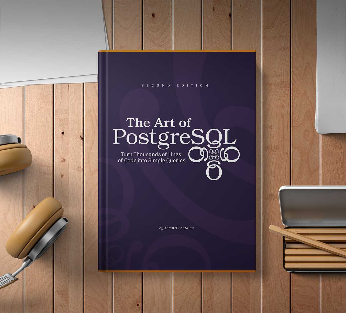
For people getting started with PostgreSQL, and SQL, the Art of PostgreSQL, by Dmitri Fontaine.
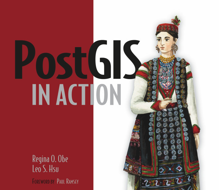
For people who are wanting to learn PostGIS, and spatial SQL, I recommend PostGIS in Action, by Regina Obe and Leo Hsu.
Both Dmitri and Regina are community members, and both have been big contributors to PostgreSQL and PostGIS. One of the key PostgreSQL features that PostGIS uses is the “extension” system, which Dmitri implemented many years ago now. And of course Regina has been active in the PostGIS develompent community almost since the first release in the early 2000s.
I often toy with the idea of writing a PostGIS or a PostgreSQL book, but then I stop and think, “wait, there’s already lots of good ones out there!” So I wrote this short post instead.
18 Nov 2019
The OGR FDW now pushes spatial filters down to remote data sources!
Whuuuut?!?!?
The Basics
OK, first, “OGR” is a subcomponent of the GDAL toolkit that allows generic access to dozens of different geospatial file formats. The OGR part handles the “vector” data (points, lines and polygons) and the GDAL part handles the “raster” data (imagery, elevation grids).
Second, “FDW” is a “foreign data wrapper”, an extension API for PostgreSQL that allows developers to connect non-database information to the database and present it in the form of a table.
The simplest FDWs, like the Oracle FDW, just make remote database tables in foreign systems look like local ones. Connecting two databases is “easy” because they share the same data model: tables of typed columns and rows of data.
The OGR data model is pleasantly similar to the database data model. Every OGR “datasource” (database) has “layers” (tables) made of “fields” (columns) with data types like “string” (varchar) and “number” (integer, real).
Now, combine the two ideas of “OGR” and “FDW”!
The “OGR FDW” uses the OGR library to present geospatial data sources as tables inside a PostgreSQL database. The FDW abstraction layer lets us make tables, and OGR abstraction layer lets those tables be sourced from almost any geospatial file format or server.
It’s an abstraction layer over an abstraction layer… the best kind!
Setup the FDW
Here’s an example that connects to a “web feature service” (WFS) from Belgium (we all speak Flemish, right?) and makes a table of it.
CREATE EXTENSION postgis;
CREATE EXTENSION ogr_fdw;

CREATE SERVER wfsserver
  FOREIGN DATA WRAPPER ogr_fdw
  OPTIONS (
    datasource 'WFS:http://geoservices.informatievlaanderen.be/overdrachtdiensten/Haltes/wfs',
    format 'WFS',
    config_options 'CPL_DEBUG=ON'
  );

CREATE FOREIGN TABLE haltes (
    fid bigint,
    shape Geometry(Point,31370),
    gml_id varchar,
    uidn double precision,
    oidn double precision,
    stopid double precision,
    naamhalte varchar,
    typehalte integer,
    lbltypehal varchar,
    codegem varchar,
    naamgem varchar
  )
  SERVER wfsserver
  OPTIONS (
    layer 'Haltes:Halte'
  );
Pushdown from FDW
Let’s run a query on the haltes table, and peak into what the OGR FDW is doing, by setting the debug level to DEBUG1.
SET client_min_messages = DEBUG1;

SELECT gml_id, ST_AsText(shape) AS shape, naamhalte, lbltypehal
  FROM haltes
  WHERE lbltypehal = 'Niet-belbus'
    AND shape && ST_MakeEnvelope(207950, 186590, 207960, 186600, 31370);
We get back one record, and two debug entries:
DEBUG:  OGR SQL: (LBLTYPEHAL = 'Niet-belbus')
DEBUG:  OGR spatial filter (207950 186590, 207960 186600)
-[ RECORD 1 ]-----------------------
gml_id     | Halte.10328
shape      | POINT(207956 186596)
naamhalte  | Lummen Frederickxstraat
lbltypehal | Niet-belbus
The debug entries are generated by the OGR FDW code, when it recognizes there are parts of the SQL query that can be passed to OGR:
- OGR understands some limited SQL syntax, and OGR FDW passes those parts of any PostgreSQL query down to OGR.
- OGR can handle simple bounding box spatial filters, and when OGR FDW sees the use of the
&& PostGIS operator, it passes the filter constant down to OGR.
So OGR FDW is passing the attribute and spatial filters from the SQL down to the OGR layer. But are they then being passed on to the remote datasource?
Pushdown from OGR
Every OGR “driver” is capable of pushing different amounts of logic down to the source data.
- A driver that reads a file format cannot push anything down: there is no logic in a file.
- A driver that reads from a database can push a lot down: databases are rich and powerful execution engines in their own right.
Our example data source, the Belgian “web feature server” actually supports both attribute and spatial filters, and the OGR driver will pass them down.
We can see OGR passing the filters down because when we created the server, we set config_options 'CPL_DEBUG=ON', to expose the GDAL logging information to our PostgreSQL server.
The GDAL debug entries are visible when we set the logging level to DEBUG2
SET client_min_messages = DEBUG2;

SELECT gml_id, ST_AsText(shape) AS shape, naamhalte, lbltypehal
  FROM haltes
  WHERE lbltypehal = 'Niet-belbus'
    AND shape && ST_MakeEnvelope(207950, 186590, 207960, 186600, 31370);
Now we get a whole slew of logging, but I’m only going to pull out one line, the line that shows the WFS query that OGR sends to the remote server:
DEBUG: GDAL None [0] WFS: http://geoservices.informatievlaanderen.be/overdrachtdiensten/Haltes/wfs?SERVICE=WFS&VERSION=1.1.0&REQUEST=GetFeature&TYPENAME=Haltes:Halte&FILTER=%3CFilter%20xmlns%3D%22http:%2F%2Fwww.opengis.net%2Fogc%22%20xmlns:Haltes%3D%22informatievlaanderen.be%2FHaltes%22%20xmlns:gml%3D%22http:%2F%2Fwww.opengis.net%2Fgml%22%3E%3CAnd%3E%3CPropertyIsEqualTo%3E%3CPropertyName%3ELBLTYPEHAL%3C%2FPropertyName%3E%3CLiteral%3ENiet%2Dbelbus%3C%2FLiteral%3E%3C%2FPropertyIsEqualTo%3E%3CBBOX%3E%3CPropertyName%3EHaltes:SHAPE%3C%2FPropertyName%3E%3Cgml:Box%3E%3Cgml:coordinates%3E207950.0000000000000000,186590.0000000000000000%20207960.0000000000000000,186600.0000000000000000%3C%2Fgml:coordinates%3E%3C%2Fgml:Box%3E%3C%2FBBOX%3E%3C%2FAnd%3E%3C%2FFilter%3E
Awesome, right?
That’s pretty much un-readable, but if I copy out the value in the FILTER request variable, and reverse the URL encoding, I get this:
<Filter
  xmlns="http://www.opengis.net/ogc"
  xmlns:Haltes="informatievlaanderen.be/Haltes"
  xmlns:gml="http://www.opengis.net/gml">
  <And>
    <PropertyIsEqualTo>
      <PropertyName>LBLTYPEHAL</PropertyName>
      <Literal>Niet-belbus</Literal>
    </PropertyIsEqualTo>
    <BBOX>
      <PropertyName>Haltes:SHAPE</PropertyName>
      <gml:Box>
        <gml:coordinates>
          207950.0000000000000000,186590.0000000000000000
          207960.0000000000000000,186600.0000000000000000
        </gml:coordinates>
      </gml:Box>
    </BBOX>
  </And>
</Filter>
I know, who ever thought that jamming an XML encoded version of a SQL filter into an HTTP GET request was a good idea? (Some very very nice people.)
Anyways, as you can see, both the attribute and spatial portions of our original SQL query have been re-encoded as a WFS XML filter, and sent to the remote server.
OGR FDW correctly pushed the attribute and spatial portions of the WHERE clause into OGR, and OGR correctly pushed those filters into the dialect of the driver we were using, in this case the WFS driver.
The End
The really really cool part is that if we had been using, for example, the Oracle driver, OGR would have instead generated Oracle-compatible SQL and pushed that down!
It’s an abstraction layer over an abstraction layer… the best kind!
13 Nov 2019
This post originally appeared in the CARTO blog.
One of the things that makes managing geospatial data challenging is the huge variety of scales that geospatial data covers: areas as large as a continent or as small as a man-hole cover.
The data in the database also covers a wide range, from single points, to polygons described with thousands of vertices. And size matters! A large object takes more time to retrieve from storage, and more time to run calculations on.
The Natural Earth countries file is a good example of that variation. Load the data into PostGIS and inspect the object sizes using SQL:
SELECT admin, ST_NPoints(the_geom), ST_MemSize(the_geom)
FROM ne_10m_admin_0_countries
ORDER BY ST_NPoints;
- Coral Sea Islands are represented with a 4 point polygon, only 112 bytes.
- Canada is represented with a 68159 point multi-polygon, 1 megabytes in size!
Over half (149) of the countries in the table are larger than the database page size (8Kb) which means they will take extra time to retrieve.
SELECT Count(*)
FROM ne_10m_admin_0_countries
WHERE ST_MemSize(the_geom) > 8192;
We can see the overhead involved in working with large data by forcing a large retrieval and computation.
Load the Natural Earth populated places into PostGIS as well, and then run a full spatial join between the two tables:
SELECT Count(*)
FROM ne_10m_admin_0_countries countries
JOIN ne_10m_populated_places_simple places
ON ST_Contains(countries.the_geom, places.the_geom)
Even though the places table (7322) and countries table (255) are quite small the computation still takes several seconds (about 30 seconds on my computer).
The large objects cause a number of inefficiencies:
- Geographically large areas (like Canada or Russia) have large bounding boxes, so the indexes don’t work as efficiently in winnowing out points that don’t fall within the countries.
- Physically large objects have large vertex lists, which take a long time to pass through the containment calculation. This combines with the poor winnowing to make a bad situation worse.
How can we speed things up? Make the large objects smaller using ST_Subdivide()!
First, generate a new, sub-divided countries table:
CREATE TABLE ne_10m_admin_0_countries_subdivided AS
SELECT ST_SubDivide(the_geom) AS the_geom, admin
FROM ne_10m_admin_0_countries;
Now we have the same data, but no object is more than 255 vertices (about 4Kb) in size!
Run the spatial join torture test again, and see the change!
SELECT Count(*)
FROM ne_10m_admin_0_countries_subdivided countries
JOIN ne_10m_populated_places_simple places
ON ST_Contains(countries.the_geom, places.the_geom)
On my computer, the return time about 0.5 seconds, or 60 times faster, even though the countries table is now 8633 rows. The subdivision has accomplished two things:
- Each polygon now covers a smaller area, so index searches are less likely to pull up points that are not within the polygon.
- Each polygon is now below the page size, so retrieval from disk will be much faster.
Subdividing big things can make map drawing faster too, but beware: once your polygons are subdivided you’ll have turn off the polygon outlines to avoid showing the funny square boundaries in your rendered map.
Happy mapping and querying!
06 Nov 2019
I love PostgreSQL extensions.
Extensions are the truest expression of the second principle of the original “design of Postgres” vision, to
provide user extendibility for data types, operators and access methods.
Extensions allow users to do more with PostgreSQL than just basic storage and retrieval. PostgreSQL is a full-on integration environment, like Python or Perl, and you can build very complete data manipulation pipelines very close to the metal using native and extension features of PostgreSQL.
Even though I’m a contributor to one of the largest PostgreSQL extensions, I have particularly come to love small extensions, that do one simple thing, particularly one simple thing we maybe take for granted in other environments.
My old HTTP extension is just a binding of libcurl to a SQL interface, so users can do web queries inside the SQL environment.
And today I’ve finished up a GZIP extension, that is just a binding of zlib to SQL, so that users can… compress and decompress things.
It’s not a lot, but it’s a little.
The GZIP entension came about because of an email on the PostGIS development list, where Yuri noted
The amazing ST_AsMVT() has two common usage patterns: copy resulting MVTs to
a tile cache (e.g. .mbtiles file or a materialized view), or serve MVT to
the users (direct SQL->browser approach). Both patterns still require one
additional data processing step – gziping.
Huh. And this use case also applies to people generating GeoJSON directly in the database and sending it out to web clients.
The PostgreSQL core has generally frowned on compression functions at the SQL level, because the database already does compression of over-sized tuples as necessary. The last thing we want is people manually applying compression to column values, and then stuffing them into rows where the database will then have to re-compress them internally. From the perspective of storage efficiency, just standing back and letting PostgreSQL do its work is preferable.
But from the perspective of an integration environment, where an application might be expected to emit or consume compressed data, having a tool in SQL to pack and unpack that data is potentially quite useful.
So I did the tiny binding to zlib and packed it up in an extension.
I hope lots of people find it useful.
26 Aug 2019
While PostGIS includes lots of algorithms and functionality we have built ourselves, it also adds geospatial smarts to PostgreSQL by linking in specialized libraries to handle particular problems:
- Proj for coordinate reference support;
- GDAL for raster functions and formats;
- GEOS for computational geometry (basic operations);
- CGAL for more computational geometry (3D operations); and
- for format support, libxml2, libjsonc, libprotobuf-c
Many of the standard geometry processing functions in PostGIS are actually evaluated inside the GEOS library, so updates in GEOS are very important to PostGIS – they add new functionality or smooth the behaviour of existing functions.
Functions backed by GEOS include:
These functions are all “overlay operation” functions – they take in geometry arguments and construct new geometries for output. Under the covers is an operation called an “overlay”, which combines all the edges of the inputs into a graph and then extracts new outputs from that graph.
While the “overlay operations” in GEOS are very reliable, they are not 100% reliable. When operations fail, the library throws the dreaded TopologyException, which indicates the graph is in an inconsistent and unusable state.
Because there are a lot of PostGIS users and they manage a lot of data, there are a non-zero number of cases that cause TopologyExceptions, and upset users. We would like take that number down to zero.
Update: Next-generation overlay did not make the 3.8 GEOS release and will be part of 3.9 instead.
With luck, GEOS 3.8 will succeed in finally bringing fully robust overlay operations to the open source community. The developer behind the GEOS algorithms, Martin Davis, recently joined Crunchy Data, and has spent this summer working on a new overlay engine.
Overlay failures are caused when intersections between edges result in inconsistencies in the overlay graph. Even using double precision numbers, systems have only 51 bits of precision to represent coordinates, and that fixed precision can result in graphs that don’t correctly reflect their inputs.
The solution is building a system that can operate on any fixed precision and retain valid geometry. As an example, here the new engine builds valid representations of Europe at any precision, even ludicrously coarse ones.
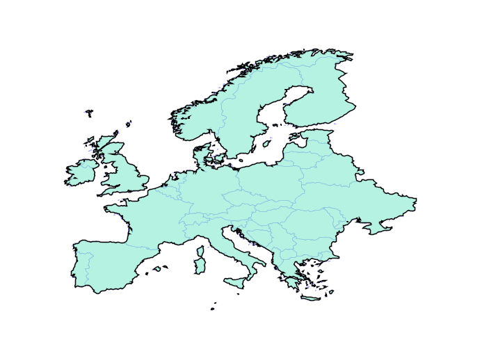
In practice, the engine will be used with a tolerance that is close to double precision, but still provides enough slack to handle tricky cases in ways that users find visually “acceptable”. Initially the new functionality should slot under the existing PostGIS functions without change, but in the future we will be able to expose knobs to allow users to explicitly set the precision domain they want to work in.
GEOS 3.8 may not be released in time for PostGIS 3, but it will be a close thing. In addition to the new overlay engine, a lot of work has been done making the code base cleaner, using more “modern” C++ idioms, and porting forward new fixes to existing algorithms.


