Parallel query has been a part of PostgreSQL since 2016 with the release of version 9.6 and in theory PostGIS should have been benefiting from parallelism ever since.
In practice, the complex nature of PostGIS has meant that very few queries would parallelize under normal operating configurations – they could only be forced to parallelize using oddball configurations.
With PostgreSQL 12 and PostGIS 3, parallel query plans will be generated and executed far more often, because of changes to both pieces of software:
PostgreSQL 12 includes a new API that allows extensions to modify query plans and add index clauses. This has allowed PostGIS to remove a large number of inlined SQL functions that were previously acting as optimization barriers to the planner.
PostGIS 3 has taken advantage of the removal of the SQL inlines to re-cost all the spatial functions with much higher costs. The combination of function inlining and high costs used to cause the planner to make poor decisions, but with the updates in PostgreSQL that can now be avoided.
Increasing the costs of PostGIS functions has allowed us to encourage the PostgreSQL planner to be more aggressive in choosing parallel plans.
PostGIS spatial functions are far more computationally expensive than most PostgreSQL functions. An area computation involves lots of math involving every point in a polygon. An intersection or reprojection or buffer can involve even more. Because of this, many PostGIS queries are bottlenecked on CPU, not on I/O, and are in an excellent position to take advantage of parallel execution.
One of the functions that benefits from parallelism is the popular ST_AsMVT() aggregate function. When there are enough input rows, the aggregate will fan out and parallelize, which is great since ST_AsMVT() calls usually wrap a call to the expensive geometry processing function, ST_AsMVTGeom().
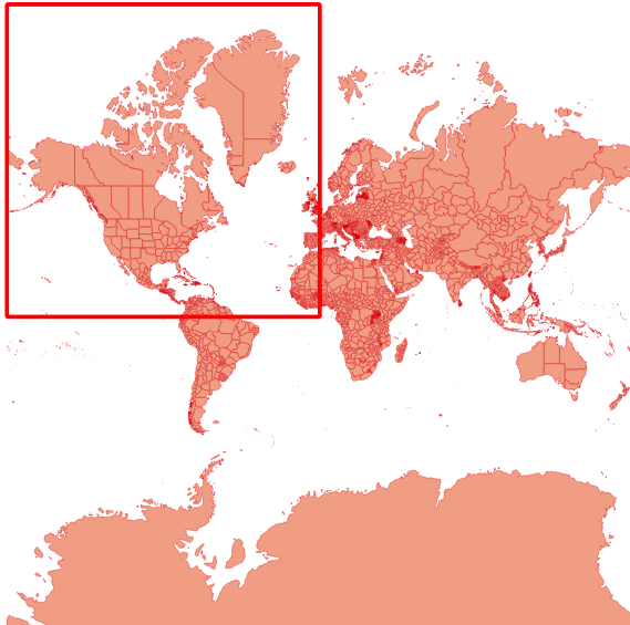
Using the Natural Earth Admin 1 layer of states and provinces as an input, I ran a small performance test, building a vector tile for zoom level one.
Spatial query performance appears to scale about the same as non-spatial as the number of cores increases, taking 30-50% less time with each doubling of processors, so not quite linearly.
Join, aggregates and scans all benefit from parallel planning, though since the gains are sublinear there’s a limit to how much performance you can extract from an operation by throwing more processors at at. Also, operations that do a large amount of computation within a single function call, like ST_ClusterKMeans, do not automatically parallelize: the system can only parallelize the calling of functions multiple times, not the internal workings of single functions.
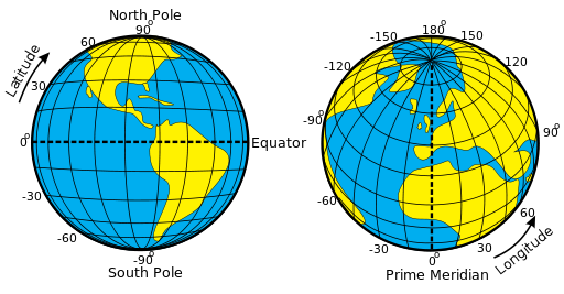
Where are you? Go ahead and figure out your answer, I’ll wait.
No matter what your answer, whether you said “sitting in my office chair” or “500 meters south-west of city hall” or “48.43° north by 123.36° west”, you expressed your location relative to something else, whether that thing was your office layout, your city, or Greenwich.
A geospatial database like PostGIS has to have able to convert between these different reference frames, known as “coordinate reference systems”. The math for these conversions and the definition of the standards needed to align them all is called “geodesy”, a field with sufficient depth and detail that you can make a career out of it.
Fortunately for users of PostGIS, most of the complexity of geodesy is hidden under the covers, and all you need to know is that different common coordinate reference systems are described in the spatial_ref_sys table, so making conversions between reference system involves knowing just two numbers: the srid (spatial reference id) of your source reference system, and the srid of your target system.
PostGIS makes use of the Proj library for coordinate reference system conversions, and PostGIS 3 will support the latest Proj release, version 6.
Proj 6 includes support for time-dependent datums and for direct conversion between datums. What does that mean? Well, one of the problems with the earth is that things move. And by things, I mean the ground itself, the very things we measure location relative to.
As location measurement becomes more accurate, and expectations for accuracy grow, reference shifts that were previously dealt with every 50 years have to be corrected closer to real time.
North America had two datums set in the twentieth century, NAD 27 and NAD 83. In 2022, North America will get new datums, fixed to the tectonic plates that make up the continent, and updated regularly to account for continental drift.
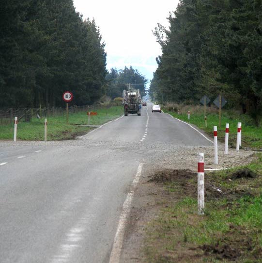
Australia is on fast moving plates that travel about 7cm per year, and will modernize its datums in 2020. 7cm/year may not sount like much, but that means that a coordinate captured to centimeter accuracy will be almost a meter out of place in a decade. For an autonomous drone navigating an urban area, that could be the difference between an uneventful trip and a crash.
Being able to accurately convert between local reference frames, like continental datums where static data are captured, to global frames like those used by the GPS/GLONASS/Galileo systems is critical for accurate and safe geo-spatial calculations.
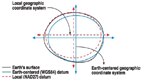
Proj 6 combines updates to handle the new frames, along with computational improvements to make conversions between frames more accurate. Older versions used a “hub and spoke” system for conversions between systems: all conversions had WGS84 as a “neutral” frame in the middle.
A side effect of using WGS84 as a pivot system was increased error, because no conversion between reference systems is error free: a conversion from one frame to another would accrue the error associated with two conversions, instead of one. Additionally, local geodesy agencies–like NOAA in the USA and GeoScience Australia–published very accurate direct transforms between historical datums, like NAD27 and NAD83, but old versions of Proj relied on hard-coded hacks to enable direct transforms. Proj 6 automatically finds and uses direct system-to-system transforms where they exist, for the most accurate possible transformation.
With the availability of MVT tile format in PostGIS via ST_AsMVT(), more and more people are generating tiles directly from the database. Doing so usually involves a couple common steps:
converting tile coordinates to ground coordinates to drive tile generation
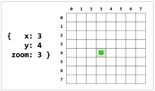
Tile coordinates consist of three values:
zoom, the level of the tile pyramid the tile is from
x, the coordinate of the tile at that zoom, counting from the left, starting at zero
y, the coordinate of the tile at that zoom, counting from the top, starting at zero
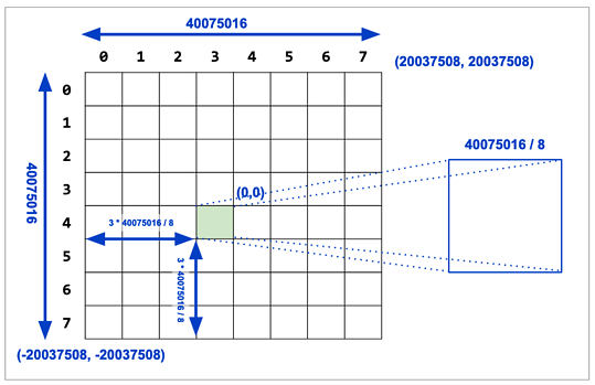
Most tile coordinates reference tiles built in the “spherical mercator” projection, which is a planar project that covers most of the world, albeit with substantial distance distortions the further north you go.
Knowing the zoom level and tile coordinates, the math to find the tile bounds in web mercator is fairly straightforward.
Most of the people generating tiles from the database write their own smallwrapper to convert from tile coordinate to mercator, as we demonstrated in a blog post last month.
It seems duplicative for everyone to do that, so we have added a utility function: ST_TileEnvelope()
By default, ST_TileEnvelope() takes in zoom, x and y coordinates and generates bounds in Spherical Mercator.
If you need to generate tiles in another coordinate system – a rare but not impossible use case – you can swap in a different spatial reference system and tile set bounds via the bounds parameter, which can encode both the tile plane bounds and the spatial reference system in a geometry:
The raster functionality in PostGIS has been part of the main extension since it was introduced. When PostGIS 3 is released, if you want raster functionality you will need to install both the core postgis extension, and also the postgis_raster extension.
Breaking out the raster functionality allows packagers to more easily build stripped down “just the basics” PostGIS without also building the raster dependencies, which include the somewhat heavy GDAL library.
The raster functionality remains intact however, and you can still do nifty things with it.
For example, download and import a “digital elevation model” file from your local government. In my case, a file that covers the City of Vancouver.
# Make a new working database and enable postgis + raster
createdb yvr_raster
psql -c'CREATE EXTENSION postgis' yvr_raster
psql -c'CREATE EXTENSION postgis_raster' yvr_raster
# BC open data from https://pub.data.gov.bc.ca/datasets/175624/# Download the DEM file, unzip and load into the database
wget https://pub.data.gov.bc.ca/datasets/175624/92g/092g06_e.dem.zip
unzip 092g06_e.dem.zip
# Options: create index, add filename to table, SRID is 4269, use 56x56 chip size
raster2pgsql -I-F-s 4269 -t 56x56 092g06_e.dem dem092g06e | psql yvr_raster
After the data load, we have a table of 56-by-56 pixel elevation chips named dem092g06e. If you map the extents of the chips, they look like this:
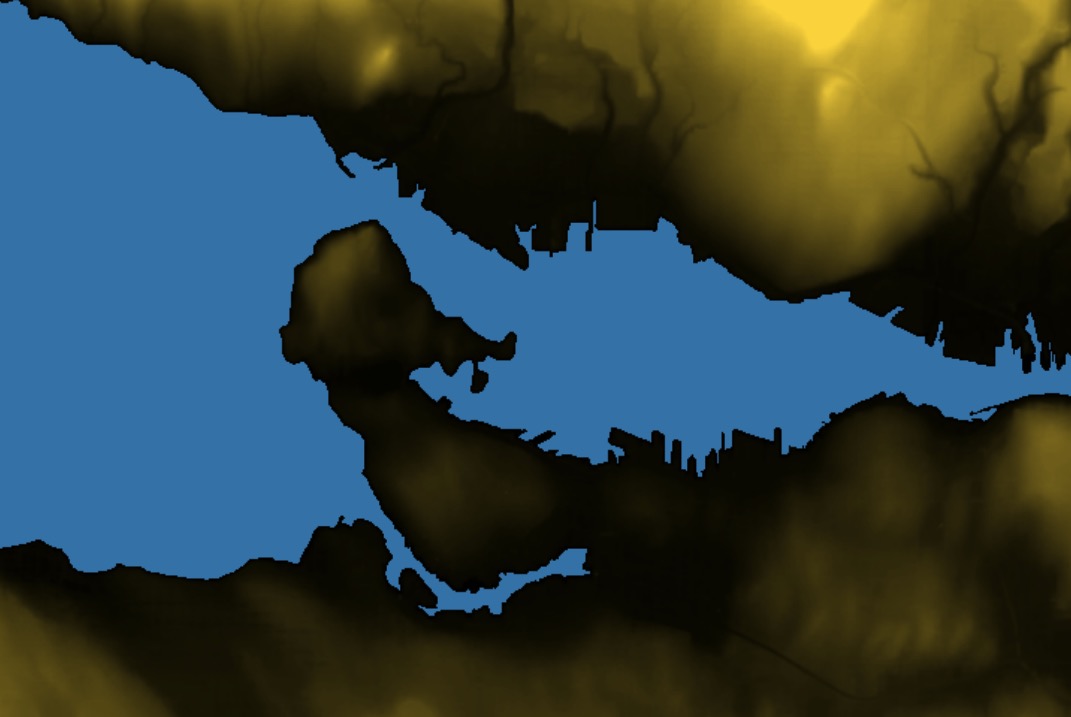
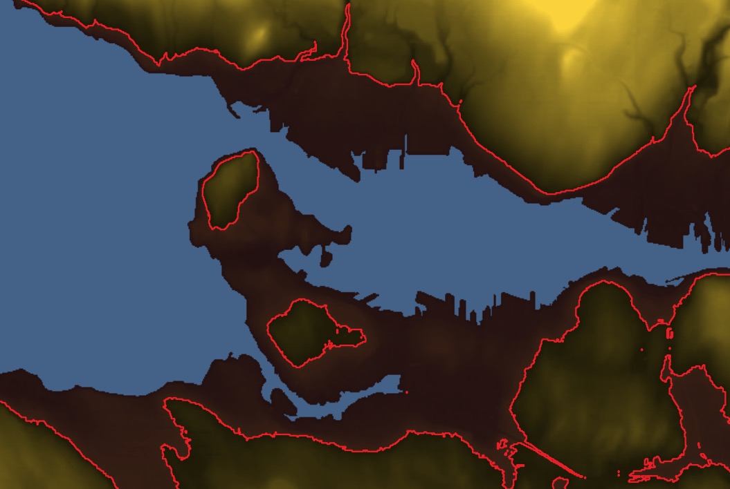
Imagine a sealevel rise of 30 meters (in an extreme case, Greenland plus Antarctica would be 68 meters). How much of Vancouver would be underwater? It’s mostly a hilly place. Let’s find out.
There are a lot of nested functions, so reading from the innermost, we:
union all the chips together into one big raster
reclassify all values from 0-30 to 1, and all higher values to 0
set the “nodata” value to 0, we don’t care about things that are above our threshold
create a vector polygon for each value in the raster (there only one value: “1”)
The result looks like this:
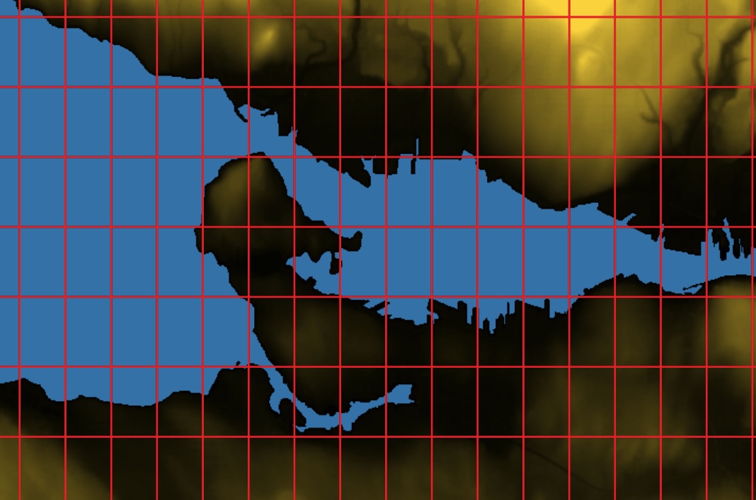
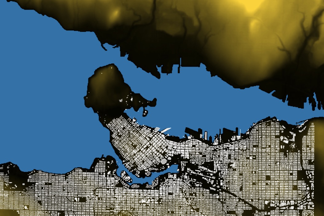
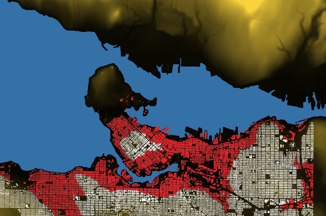
We can grab building footprints for Vancouver and see how many buildings are going to be underwater.
# Vancouver open data # https://data.vancouver.ca/datacatalogue/buildingFootprints.htm
wget ftp://webftp.vancouver.ca/OpenData/shape/building_footprints_2009_shp.zip
unzip building_footprints_2009_shp.zip
# Options: create index, SRID is 26910, use dump format
shp2pgsql -I-s 26910 -D building_footprints_2009 buildings | psql yvr_raster
Before we can compare the buildings to the flood zone, we need to put them into the same projection as the flood zone (SRID 4269).
(There are buildings on the north shore of Burrard inlet, but this data is from the City of Vancouver. Jurisdictional boundaries are the bane of geospatial analysis.)
There’s another way to find buildings below 30 meters, without having to build a polygon: just query the raster value underneath each building, like this:
Vector tiles are the new hotness, allowing large amounts of dynamic data to be sent for rendering right on web clients and mobile devices, and making very beautiful and highly interactive maps possible.
Since the introduction of ST_AsMVT(), people have been generating their tiles directly in the database more and more, and as a result wanting tile generation to go faster and faster.
Every tile generation query has to carry out the following steps:
Gather all the relevant rows for the tile
Simplify the data appropriately to match the resolulution of the tile
For PostGIS 3.0, performance of tile generation has been vastly improved.
First, the clipping process has been sped up and made more reliable by integrating the wagyu clipping algorithm directly into PostGIS. This has sped up clipping of polygons in particular, and reduced instances of invalid output geometries.
Second, the simplification and precision reduction steps have been streamlined, to avoid unnecessary copying and work on simple cases like points and short lines. This has sped up handling of simple points and lines.
Finally, ST_AsMVT() aggregate itself has been made parallelizeable, so that all the work above can be parcelled out to multiple CPUs, dramatically speeding up generation of tiles with lots of input geometry.
PostGIS vector tile support has gotten so good that even projects with massive tile generation requirements, like the OpenMapTiles project, have standardized their tiling on PostGIS.