20 Aug 2019
With the release of PostGIS 3.0, queries that ORDER BY geometry columns will return rows using a Hilbert curve ordering, and do so about twice as fast.
Whuuuut!?!
The history of “ordering by geometry” in PostGIS is mostly pretty bad. Up until version 2.4 (2017), if you did ORDER BY on a geometry column, your rows would be returned using the ordering of the minimum X coordinate value in the geometry.
One of the things users expect of “ordering” is that items that are “close” to each other in the ordered list should also be “close” to each other in the domain of the values. For example, in a set of sales orders ordered by price, rows next to each other have similar prices.
To visualize what geometry ordering looks like, I started with a field of 10,000 random points.
CREATE SEQUENCE points_seq;

CREATE TABLE points AS
SELECT
  (ST_Dump(
    ST_GeneratePoints(
        ST_MakeEnvelope(-10000,-10000,10000,10000,3857),
        10000)
    )).geom AS geom,
  nextval('points_seq') AS pk;

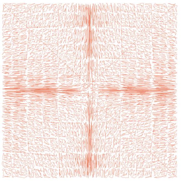
Now select from the table, and use ST_MakeLine() to join them up in the desired order. Here’s the original ordering, prior to version 2.4.
SELECT ST_MakeLine(geom ORDER BY ST_X(geom)) AS geom
FROM points;

Each point in the ordering is close in the X coordinate, but since the Y coordinate can be anything, there’s not much spatial coherence to the ordered set. A better spatial ordering will keep points that are near in space also near in the set.
For 2.4 we got a little clever. Instead of sorting by the minimum X coordinate, we took the center of the geomery bounds, and created a Morton curve out of the X and Y coordinates. Morton keys just involve interleaving the bits of the values on the two axes, which is a relatively cheap operation.
The result is way more spatially coherent.
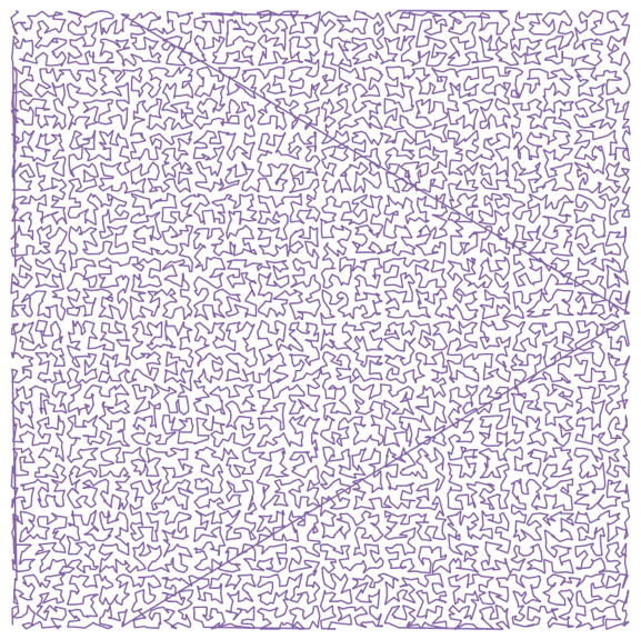
For 3.0, we have replaced the Morton curve with a Hilbert curve. The Hilbert curve is slightly more expensive to calculate, but we offset that by stripping out some wasted cycles in other parts of the old implementation, and the new code is now faster, and also even more spatially coherent.
SELECT ST_MakeLine(geom ORDER BY geom) AS geom
FROM points;
PostGIS 3.0 will be released some time this fall, hopefully before the final release of PostgreSQL 12.
19 Aug 2019
With PostGIS 3.0, it is now possible to generate GeoJSON features directly without any intermediate code, using the new ST_AsGeoJSON(record) function.
The GeoJSON format is a common transport format, between servers and web clients, and even between components of processing chains. Being able to create useful GeoJSON is important for integrating different parts in a modern geoprocessing application.
PostGIS has had an ST_AsGeoJSON(geometry) for forever, but it does slightly less than most users really need: it takes in a PostGIS geometry, and outputs a GeoJSON “geometry object”.
The GeoJSON geometry object is just the shape of the feature, it doesn’t include any of the other information about the feature that might be included in the table or query. As a result, developers have spent a lot of time writing boiler-plate code to wrap the results of ST_AsGeoJSON(geometry) up with the columns of a result tuple to create GeoJSON “feature objects”.
The ST_AsGeoJSON(record) function looks at the input tuple, and takes the first column of type geometry to convert into a GeoJSON geometry. The rest of the columns are added to the GeoJSON features in the properties member.
SELECT ST_AsGeoJSON(subq.*) AS geojson
FROM (
  SELECT ST_Centroid(geom), type, admin
  FROM countries
  WHERE name = 'Canada'
) AS subq
{"type": "Feature",
 "geometry": {
    "type":"Point",
    "coordinates":[-98.2939042718784,61.3764628013483]
  },
  "properties": {
    "type": "Sovereign country",
    "admin": "Canada"
  }
}
Using GeoJSON output it’s easy to stream features directly from the database into an OpenLayers or Leaflet web map, or to consume them with ogr2ogr for conversion to other geospatial formats.
16 Aug 2019
The years keep on ticking by, but the numbers never get any smaller. The contracts are written for decades at a time, and change is hard so…?
In the UK, the review of IT outsourcing contracts was called the “Ocean Liner report”, with reference to how long it takes to turn one around.
That said, the curve of BC outsourced IT spending continues to march upward.

To what do we owe the continued growth? This year, no one vendor can really claim the lion’s share of growth, and yet every vendor except Maximus notched some modest growth. I would expect the $79M Maximus revenue line to shrink pretty quickly over the next couple years, as the MSP billing system winds down.

Maximus revenue won’t go to zero though. Having built out the infrastructure for collecting MSP premiums, they took that expertise and won contracts to collect court ordered family support payments. That vendor relationship got so intertwined with the Ministry that the Auditor General looked askance at it. They also used their position in the data flow to ramp up billings by taking on more responsibilities and adding to their systems.
This is one of the reasons that billings tend to go up-and-up even though outsourcing contracts are usually justified in the name of cost control and predictability.
From a vendor point of view, the beauty of an outsourcing agreement is that it lands you into the heart of a business, providing a privileged view of the opportunity space. There is nothing a client likes more (assuming they have the budget) then a vendor that can pro-actively provide a proposal to fix an obvious business problem. The fact that the visibility into those problems is monopolized by the incumbent vendor is just an unfortunate side effect. Over time, these little proposals can grow into whole new lines of outsourced work. If there is no internal capacity to support the new programs, the vendor just increases its share of government revenues.
The UK is as big and complex as BC (more so, of course) and they have reviewed their major outsourcing contracts, and exited a few. Iain Patterson, who wrote the “Ocean Liner” report, saw incumbent vendors, and their bias towards the (lucrative) status quo as a barrier to modernization:
Unfortunately, the main barrier that prevents departments from investing in these solutions is the contract landscape. Many still have large, legacy contracts using system integrators which affect their ability to change their technology estate. They’re faced with costly change control requests and complicated workarounds to link up cloud-based commodity solutions with their existing technology.
Unfortunately, there is no one answer to how to get out of the bind, except “very slowly and carefully”. As Patterson said:
“Understand the capabilities you have,” he said. “Understand what you’ve got as far as your contractual commitments. When the contracts expire, work with the companies that hold those contracts to try and change that landscape during the lifetime of the contract.
“And if you can’t do that, then we will try to do things in a different way. But we’ll come out of those contracts understanding what it is that we have in them at that moment in time, what can we commoditise in those, and where they are best suited to be delivered from, whether that’s internal, external, or whether there are things we can buy now rather than build.”
Turn that ocean liner, a little bit at a time.
31 Jul 2019
And, late on a Friday afternoon, the plaintive cry was heard!
And indeed, into the sea they do go!
And ‘lo, the SQL faeries were curious, and gave it a shot!
##### Commandline OSX/Linux #####

# Get the Shape files
# http://www.elections.bc.ca/index.php/voting/electoral-maps-profiles/
wget http://www.elections.bc.ca/docs/map/redis08/GIS/ED_Province.exe

# Exe? No prob, it's actually a self-extracting ZIP
unzip ED_Province

# Get a PostGIS database ready for the data
createdb ed_clip
psql -c "create extension postgis" -d ed_clip

# Load into PostGIS
# The .prj says it is "Canada Albers Equal Area", but they
# lie! It's actually BC Albers, EPSG:3005
shp2pgsql -s 3005 -i -I ED_Province ed | psql -d ed_clip

# We need some ocean! Use Natural Earth...
# http://www.naturalearthdata.com/downloads/
wget http://www.naturalearthdata.com/http//www.naturalearthdata.com/download/10m/physical/ne_10m_ocean.zip
unzip ne_10m_ocean.zip

# Load the Ocean into PostGIS!
shp2pgsql -s 4326 -i -I ne_10m_ocean ocean | psql -d ed_clip

# OK, now we connect to PostGIS and start working in SQL
psql -e ed_clip
-- How big is the Ocean table?
SELECT Count(*) FROM ocean;

-- Oh, only 1 polygon. Well, that makes it easy...
-- For each electoral district, we want to difference away the ocean.
-- The ocean is a one big polygon, this will take a while (if we
-- were being more subtle, we'd first clip the ocean down to
-- a reasonable area around BC.)
CREATE TABLE ed_clipped AS
SELECT
  CASE
  WHEN ST_Intersects(o.geom, ST_Transform(e.geom,4326))
  THEN ST_Difference(ST_Transform(e.geom,4326), o.geom)
  ELSE ST_Transform(e.geom,4326)
  END AS geom,
  e.edabbr,
  e.edname
FROM ed e, ocean o;

-- Check our geometry types...
SELECT DISTINCT ST_GeometryType(geom) FROM ed_clipped;

-- Oh, they are heterogeneous. Let's force them all multi
UPDATE ed_clipped SET geom = ST_Multi(geom);
# Dump the result out of the database back into shapes
pgsql2shp -f ed2009_ocean ed_clip ed_clipped
zip ed2009_ocean.zip ed2009_ocean.*
mv ed2009_ocean.zip ~/Dropbox/Public/
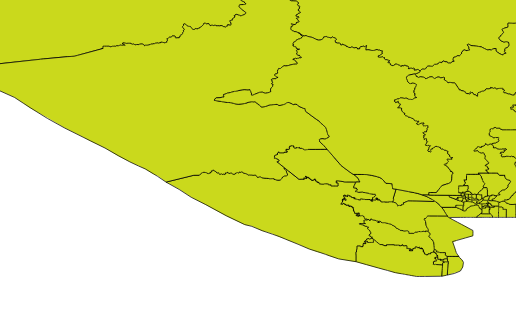
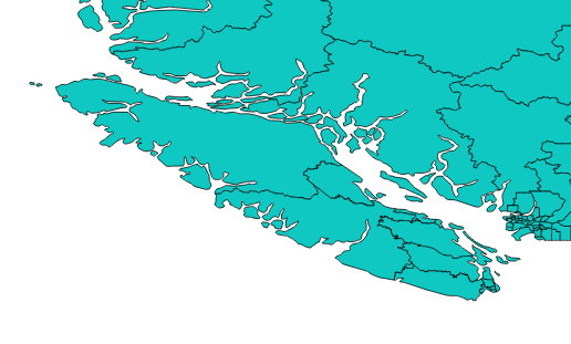
No more districts in oceans!
And the faeries were happy, and uploaded their polygons!
Update: And the lamentations ended, and the faeries also rejoiced.
30 Jul 2019
One question that comes up often during our PostGIS training is “how do I do an overlay?” The terminology can vary: sometimes they call the operation a “union” sometimes an “intersect”. What they mean is, “can you turn a collection of overlapping polygons into a collection of non-overlapping polygons that retain information about the overlapping polygons that formed them?”
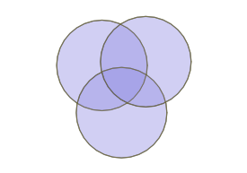
So an overlapping set of three circles becomes a non-overlapping set of 7 polygons.

Calculating the overlapping parts of a pair of shapes is easy, using the ST_Intersection() function in PostGIS, but that only works for pairs, and doesn’t capture the areas that have no overlaps at all.
How can we handle multiple overlaps and get out a polygon set that covers 100% of the area of the input sets? By taking the polygon geometry apart into lines, and then building new polygons back up.
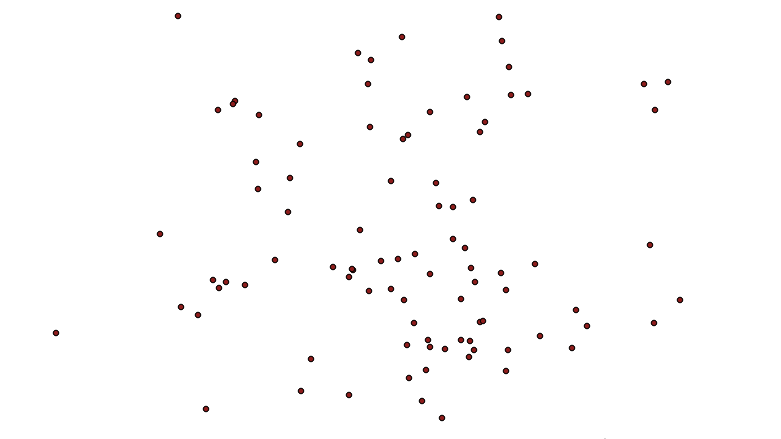
Let’s construct a synthetic example: first, generate a collection of random points, using a Gaussian distribution, so there’s more overlap in the middle. The crazy math in the SQL below just converts the uniform random numbers from the random() function into normally distributed numbers.
CREATE TABLE pts AS
  WITH rands AS (
  SELECT generate_series as id,
         random() AS u1,
         random() AS u2
  FROM generate_series(1,100)
)
SELECT
  id,
  ST_SetSRID(ST_MakePoint(
    50 * sqrt(-2 * ln(u1)) * cos(2*pi()*u2),
    50 * sqrt(-2 * ln(u1)) * sin(2*pi()*u2)), 4326) AS geom
FROM rands;
The result looks like this:
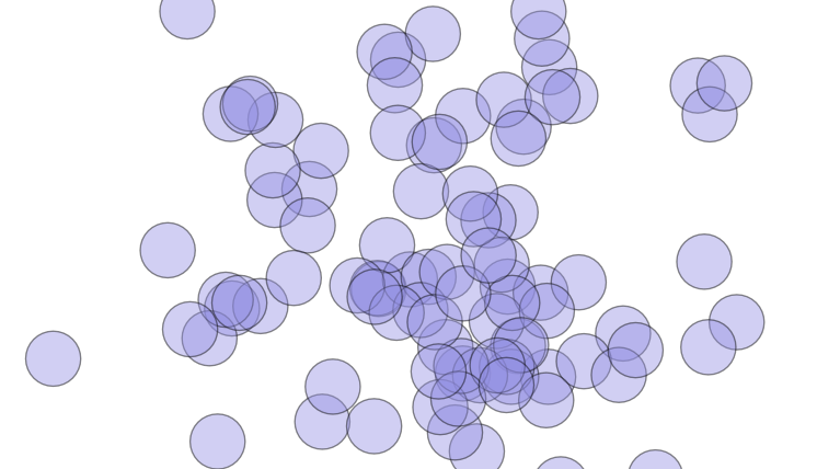
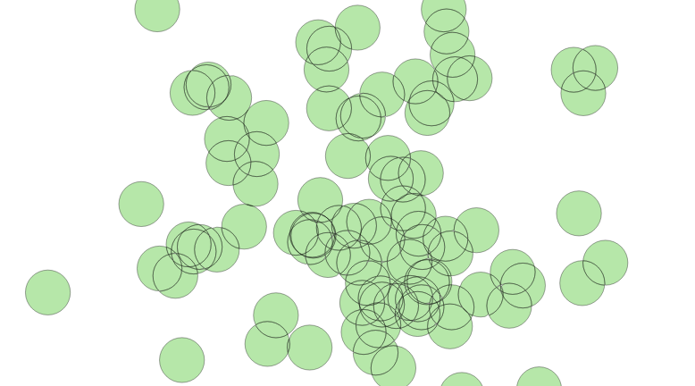
Now, we turn the points into circles, big enough to have overlaps.
CREATE TABLE circles AS
  SELECT id, ST_Buffer(geom, 10) AS geom
    FROM pts;
Which looks like this:
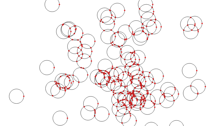
Now it’s time to take the polygons apart. In this case we’ll take the exterior ring of the circles, using ST_ExteriorRing(). If we were dealing with complex polygons with holes, we’d have to use ST_DumpRings(). Once we have the rings, we want to make sure that everywhere rings cross the lines are broken, so that no lines cross, they only touch at their end points. We do that with the ST_Union() function.
CREATE TABLE boundaries AS
  SELECT ST_Union(ST_ExteriorRing(geom)) AS geom
    FROM circles;
What comes out is just lines, but with end points at every crossing.
Now that we have noded lines, we can collect them into a multi-linestring and feed them to ST_Polygonize() to generate polygons. The polygons come out as one big multi-polygon, so we’ll use ST_Dump() to convert it into a table with one row per polygon.
CREATE SEQUENCE polyseq;
CREATE TABLE polys AS
  SELECT nextval('polyseq') AS id,
         (ST_Dump(ST_Polygonize(geom))).geom AS geom
  FROM boundaries;
Now we have a set of polygons with no overlaps, only one polygon per area.
So, how do we figure out how many overlaps contributed to each incoming polygon? We can join the centroids of the new small polygons with the set of original circles, and calculate how many circles contain each centroid point.
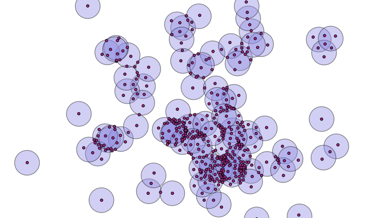
A spatial join will allow us to calculate the number of overlaps.
ALTER TABLE polys ADD COLUMN count INTEGER DEFAULT 0;
UPDATE POLYS set count = p.count
FROM (
  SELECT count(*) AS count, p.id AS id
  FROM polys p
  JOIN circles c
  ON ST_Contains(c.geom, ST_PointOnSurface(p.geom))
  GROUP BY p.id
) AS p
WHERE p.id = polys.id;
That’s it! Now we have a single coverage of the area, where each polygon knows how much overlap contributed to it. Ironically, when visualized using the coverage count as a variable in the color ramp, it looks a lot like the original image, which was created with a simple transparency effect. However, the point here is that we’ve created new data, in the count attribute of the new polygon layer.
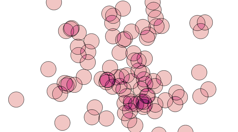
The same decompose-and-rebuild-and-join-centroids trick can be used to overlay all kinds of features, and to carry over attributes from the original input data, achieving the classic “GIS overlay” workflow. Happy geometry mashing!


