Update: See below, but I didn’t test the full pushdown case, and the result is pretty awesome.
I have been wondering for a while if Postgres would correctly plan a spatial join over FDW, in which one table was local and one was remote. The specific use case would be “keeping a large pile of data on one side of the link, and joining to it”.
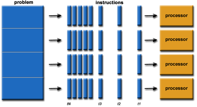
Because spatial joins always plan out to a “nested loop” execution, where one table is chosen to drive the loop, and the other to be filtered on the rows from the driver, there’s nothing to prevent the kind of remote execution I was looking for.
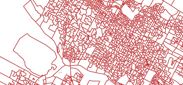
I set up my favourite spatial join test: BC voting areas against BC electoral districts, with local and remote versions of both tables.
CREATEEXTENSIONpostgres_fdw;-- Loopback foreign server connects back to-- this same databaseCREATESERVERtestFOREIGNDATAWRAPPERpostgres_fdwOPTIONS(host'127.0.0.1',dbname'test',extensions'postgis');CREATEUSERMAPPINGFORpramseySERVERtestOPTIONS(user'pramsey',password'');-- Foreign versions of the local tables CREATEFOREIGNTABLEed_2013_fdw(gidinteger,ednametext,edabbrtext,geomgeometry(MultiPolygon,4326))SERVERtestOPTIONS(table_name'ed_2013',use_remote_estimate'true');CREATEFOREIGNTABLEva_2013_fdw(gidintegerOPTIONS(column_name'gid'),idtextOPTIONS(column_name'id'),vaabbrtextOPTIONS(column_name'vaabbr'),edabbrtextOPTIONS(column_name'edabbr'),geomgeometry(MultiPolygon,4326)OPTIONS(column_name'geom'))SERVERtestOPTIONS(table_name'va_2013',use_remote_estimate'true');
The key option here is use_remote_estimate set to true. This tells postgres_fdw to query the remote server for an estimate of the remote table selectivity, which is then fed into the planner. Without use_remote_estimate, PostgreSQL will generate a terrible plan that pulls the contents of the `va_2013_fdw table local before joining.
With use_remote_estimate in place, the plan is just right:
GroupAggregate  (cost=241.14..241.21 rows=2 width=12)
 Output: count(*), e.edabbr
 Group Key: e.edabbr
 ->  Sort  (cost=241.14..241.16 rows=6 width=4)
     Output: e.edabbr
     Sort Key: e.edabbr
     ->  Nested Loop  (cost=100.17..241.06 rows=6 width=4)
         Output: e.edabbr
         ->  Seq Scan on public.ed_2013 e  (cost=0.00..22.06 rows=2 width=158496)
             Output: e.gid, e.edname, e.edabbr, e.geom
             Filter: ((e.edabbr)::text = ANY ('{VTB,VTS}'::text[]))
         ->  Foreign Scan on public.va_2013_fdw v  (cost=100.17..109.49 rows=1 width=4236)
             Output: v.gid, v.id, v.vaabbr, v.edabbr, v.geom
             Remote SQL: SELECT geom FROM public.va_2013 WHERE (($1::public.geometry(MultiPolygon,4326) OPERATOR(public.&&) geom)) AND (public._st_intersects($1::public.geometry(MultiPolygon,4326), geom))
For FDW drivers other than postgres_fdw this means there’s a benefit to going to the trouble to support the FDW estimation callbacks, though the lack of exposed estimation functions in a lot of back-ends may mean the support will be ugly hacks and hard-coded nonsense. PostgreSQL is pretty unique in exposing fine-grained information about table statistics.
Update
One “bad” thing about the join pushdown plan above is that it still pulls all the resultant records back to the source before aggregating them, so there’s a missed opportunity there. However, if both the tables in the join condition are remote, the system will correctly plan the query as a remote join and aggregation.
One of the core complaints in my review of PostgreSQL parallelism, was that the cost of functions executed on rows returned by queries do not get included in evaluations of the cost of a plan.
So for example, the planner appeared to consider these two queries equivalent:
SELECT*FROMpd;SELECTST_Area(geom)FROMpd;
They both retrieve the same number of rows and both have no filter on them, but the second one includes a fairly expensive function evaluation. No amount of changing the cost of the ST_Area() function would cause a parallel plan to materialize. Only changing the size of the table (making it bigger) would flip the plan into parallel mode.
With the patch in place, I now see rational behavior from the planner. Using the default PostGIS function costs, a simple area calculation on my 60K row polling division table is sequential:
EXPLAINSELECTST_Area(geom)FROMpd;
Seq Scan on pd
(cost=0.00..14445.17 rows=69534 width=8)
However, if the ST_Area() function is costed a little more realistically, the plan shifts.
While not every query receives what I consider a “perfect plan”, it now appears that we at least have some reasonable levers available to get better plans via applying some sensible (higher) costs across the PostGIS code base.
The results at the time were mixed: parallel query worked, when poked just the right way, with the correct parameters set on the PostGIS functions, and on the PostgreSQL back-end. However, under default settings, parallel queries did not materialize. Not for scans, not for joins, not for aggregates.
With the recent release of PostgreSQL 10, another generation of improvement has been added to parallel query processing, so it’s fair to ask, “how well does PostGIS parallelize now?”
TL;DR:
The answer is, better than before:
Parallel aggregations now work out-of-the-box and parallelize in reasonable real-world conditions.
Parallel scans still require higher function costs to come into action, even in reasonable cases.
Parallel joins on spatial conditions still seem to have poor planning, requiring a good deal of manual poking to get parallel plans.
Setup
In order to run these tests yourself, you will need:
PostgreSQL 10
PostGIS 2.4
You’ll also need a multi-core computer to see actual performance changes. I used a 4-core desktop for my tests, so I could expect 4x improvements at best.
The configuration parameters for parallel query have changed since the last test, and are (in my opinion) a lot easier to understand.
These parameters are used to fine-tune the planner and execution. Usually you don’t need to change them.
parallel_setup_cost sets the planner’s estimate of the cost of launching parallel worker processes. Default 1000.
parallel_tuple_cost sets the planner’s estimate of the cost of transferring one tuple from a parallel worker process to another process. Default 0.1.
min_parallel_table_scan_size sets the minimum amount of table data that must be scanned in order for a parallel scan to be considered. Default 8MB.
min_parallel_index_scan_size sets the minimum amount of index data that must be scanned in order for a parallel scan to be considered. Default 512kB.
force_parallel_mode forces the planner to parallelize is wanted. Values: off | on | regress
effective_io_concurrency for some platforms and hardware setups allows true concurrent read. Values from 1 (for one spinning disk) to ~100 (for an SSD drive). Default 1.
These parameters control how many parallel processes are launched for a query.
max_worker_processes sets the maximum number of background processes that the system can support. Default 8.
max_parallel_workers sets the maximum number of workers that the system can support for parallel queries. Default 8.
max_parallel_workers_per_gather sets the maximum number of workers that can be started by a single Gather or Gather Merge node. Setting this value to 0 disables parallel query execution. Default 2.
Once you get to the point where #processes == #cores there’s not a lot of advantage in adding more processes. However, each process does exact a cost in terms of memory: a worker process consumes work_mem the same as any other backend, so when planning memory usage take both max_connectionsandmax_worker_processes into consideration.
Before running tests, make sure you have a handle on what your parameters are set to: I frequently found I accidentally tested with max_parallel_workers set to 1.
First, set max_parallel_workers and max_parallel_workers_per_gather to 8, so that the planner has as much room as it wants to parallelize the workload.
PostGIS only has one true spatial aggregate, the ST_MemUnion function, which is comically inefficient due to lack of input ordering. However, it’s possible to see some aggregate parallelism in action by wrapping a spatial function in a parallelizable aggregate, like Sum():
It appears our spatial function costs may still be too low in general to get good planning. And as we will see with joins, it’s possible the planner is still discounting function costs too much in deciding whether to go parallel or not.
Joins
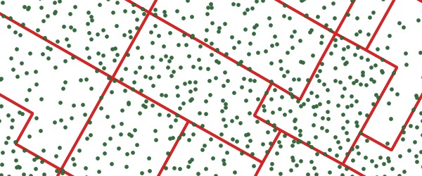
Starting with a simple join of all the polygons to the 100 points-per-polygon table, we get:
In order to give the PostgreSQL planner a fair chance, I started with the largest table, thinking that the planner would recognize that a “70K rows against 7M rows” join could use some parallel love, but no dice:
Nested Loop
(cost=0.41..13555950.61 rows=1718613817 width=2594)
 ->  Seq Scan on pd
     (cost=0.00..14271.34 rows=69534 width=2554)
 ->  Index Scan using pts_gix on pts
     (cost=0.41..192.43 rows=232 width=40)
       Index Cond: (pd.geom && geom)
       Filter: _st_intersects(pd.geom, geom)
There are a number of knobs we can press on. There are two global parameters:
parallel_setup_cost defaults to 1000, but no amount of lowering the value, even to zero, causes a parallel plan.
parallel_tuple_cost defaults to 0.1. Reducing it by a factor of 100, to 0.001 causes the plan to flip over into a parallel plan.
SETparallel_tuple_cost=0.001;
As with all parallel plans, it is a nested loop, but that’s fine since all PostGIS joins are nested loops.
Gather  (cost=0.28..4315272.73 rows=1718613817 width=2594)
Workers Planned: 4
->  Nested Loop
    (cost=0.28..2596658.92 rows=286435636 width=2594)
     ->  Parallel Seq Scan on pts_100 pts
         (cost=0.00..69534.00 rows=1158900 width=40)
     ->  Index Scan using pd_geom_idx on pd
         (cost=0.28..2.16 rows=2 width=2554)
           Index Cond: (geom && pts.geom)
           Filter: _st_intersects(geom, pts.geom)
Running the parallel plan to completion on the 700K point table takes 18s with four workers and 53s with a sequential plan. We are not getting an optimal speed up from parallel processing anymore: four workers are completing in 1/3 of the time instead of 1/4.
If we set parallel_setup_cost and parallel_tuple_cost back to their defaults, we can also change the plan by fiddling with the function costs.
First, note that our query can be re-written like this, to expose the components of the spatial join:
The overlay operation finds, for each geometry on one side, all the overlapping geometries, and then calculates the shape of those overlaps (the “intersection” of the pair). Calculating intersections is expensive, so it’s something want to happen in parallel, even more than we want the join to happen in parallel.
This query calculates the overlay of all polling divisions (and their translations) in British Columbia (fed_num > 59000):
Unfortunately, the default remains a non-parallel plan. The parallel_tuple_cost has to be adjusted down to 0.01 or the cost of _ST_Intersects() adjusted upwards to get a parallel plan.
Conclusions
The costs assigned to PostGIS functions still do not provide the planner a good enough guide to determine when to invoke parallelism. Costs assigned currently vary widely without any coherent reasons.
The planner behaviour on spatial joins remains hard to predict: is the deciding factor the join operator cost, the number of rows of resultants, or something else altogether? Counter-intuitively, it was easier to get join behaviour from a relatively small 6K x 6K polygon/polygon overlay join than it was for the 70K x 7M point/polygon overlay.
I’m yak shaving this morning, and one of the yaks I need to ensmooth is running a PHP script that connects to a PgSQL database.
No problem, OSX ships with PHP! Oh wait, that PHP does not include PgSQL database support.
At this point, you can either run to completely replace your in-build PHP with another PHP (probably good if you’re doing modern PHP development and want something newer than 5.5) or you can add PgSQL to your existing PHP installation. I chose the latter.
The key is to build the extension you want without building the whole thing. This is a nice trick available in PHP, similar to the Apache module system for independent module development.
First, figure out what version of PHP you will be extending:
Then, unbundle it and go to the php extension directory:
tar xvfz php-5.5.38.tar.bz2
cd php-5.5.38/ext/pgsql
Now the magic part. In order to build the extension, without building the whole of PHP, we need to tell the extension how the PHP that Apple ships was built and configured. How do we do that? We run phpize in the extension directory.
> /usr/bin/phpize

Configuring for:
PHP Api Version:         20121113
Zend Module Api No:      20121212
Zend Extension Api No:   220121212
The phpize process reads the configuration of the installed PHP and sets up a local build environment just for the extension. All of a sudden we have a ./configure script, and we’re ready to build (assuming you have installed the MacOSX command-line developers tools with XCode).
> ./configure \
    --with-php-config=/usr/bin/php-config \
    --with-pgsql=/opt/pgsql/10

> make
Note that I have my own build of PostgreSQL in /opt/pgsql. You’ll need to supply the path to your own install of PgSQL so that the PHP extension can find the PgSQL libraries and headers to build against.
When the build is complete, you’ll have a new modules/ directory in the extension directory. Now figure out where your system wants extensions copied, and copy the module there.
Finally, you need to edit the /etc/php.ini file to enable the new module. If the file doesn’t already exist, you’ll have to copy in the template version and then edit that.
sudo cp /etc/php.ini.default /etc/php.ini
sudo vi /etc/php.ini
Find the line for the PgSQL module and uncomment and edit it appropriately.
Now you can check and see if it has picked up the PgSQL module.
> php --info | grep PostgreSQL

PostgreSQL Support => enabled
PostgreSQL(libpq) Version => 10.0
PostgreSQL(libpq)  => PostgreSQL 10.0 on x86_64-apple-darwin15.6.0, compiled by Apple LLVM version 8.0.0 (clang-800.0.42.1)
Whoops, it snuck by me in the laze of summer, but the BC Public Accounts have come out, so I can do a (partial) update of my IT outsourcing summary. Why “partial”? Because I cannot include Health Region spending until their vendor spending summaries are released late in the year. So this summary is for central government only.
The year-over-year trend is flat, which means that last year’s steep drop-off of spending on IBM dominates the look of the chart.
The chart by vendor gives a better feel for who is up and who is down:
IBM, up a little year-over-year, but still way down after last years’ collapse. ESIT continues to dominate all vendors by a large margin. Note that ESIT is the new name for HP Advanced Solutions (HPAS) which was itself the new name for the BC operations of EDS.
Maximus is up a little, but with the MSP premium program (and thus the associated administration contract) potentially winding down it’s hard to imagine any long term trend for them but down. At a minimum the 50% cut in premium rates effectively doubles the administrative overhead represented by the Maximum contract, which is not a good look.
One thing I’m going to be looking at once the health numbers are in is whether billings by Cerner move up to compensate for the drop-off by IBM. By rights they should: Cerner has taken over the huge EHR project at PHSA/Coastal. On the other hand, I heard a rumour that much of that spending was shifted out to a “non-profit” entity by the BC Liberals, which would make it disappear from my survey of vendor payments reports.