28 Nov 2021
A couple weeks ago, former BC Liberal MLA and current radio host Jas Johal delivered an epic twitter rant trashing his former party’s record on diversity.

Among other things, he pointed out the distinctive rule the 2018 BC Liberal leadership contest was run under, which granted 100 points for each riding in the province and distributed those points based on the votes within each riding.
Even your 100 points per riding for leadership, is to reduce the impact of South Asian signups.
The net effect of the “100 point rule” is a “one riding one vote” system, rather than a “one person one vote” system.
For those of you joining from outside BC: the South Asian community in BC has an admirable history of political engagement and can wield outsize influence in contests (like leadership elections) which place a premium on signing up and activating new party members. Because the community is concentrated in a few regions, this extra activity results in a some ridings having a lot of new members during leadership contests. Normalizing votes on a per-riding basis has the effect of devaluing votes in these highly active ridings.
Johal’s rant made me wonder though: sure, the (often unspoken) conventional wisdom was that the point system devalued South Asian votes, but in the final analysis, did it?
Incredibly, the riding-by-riding vote results for the 2018 BC Liberal leadership contest are all available in Wikipedia, so it is possible to do a loose analysis.
We cannot know exactly what the visible minority make-up of the BC Liberal membership was in 2018, but we can approximate it by using the 2016 Census profiles for the ridings.
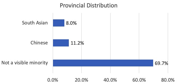
The three largest visible minority categories in BC for 2016 were “Not a visible minority”, “Chinese”, and “South Asian”, so I did analyses for these three groups.
Here’s the overall provincial distribution of those three visible minority categories:
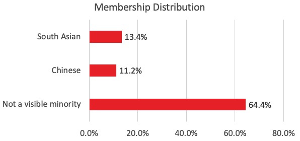
Here’s the distribution of those categories within the BC Liberal membership, calculated by weighting using the riding level distributions against the membership in each riding:
And here’s the scaled BC Liberal membership distribution, where each riding is given equal weight, as in the 100-point leadership vote counting rules.
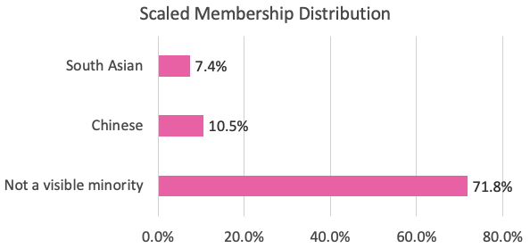
So, yeah, Johal wasn’t just making this up, the 100-point system is not only anti-democratic in conception (“one vote per riding” instead of “one vote per person”), the system disadvantages the South Asian community in particular.
Having done this lightweight analysis, it is super tempting to try and figure out the counter-factual–who would have won the 2018 leadership under a one-member-one-vote rule–but unfortunately that’s not possible with the data available.
25 Nov 2021
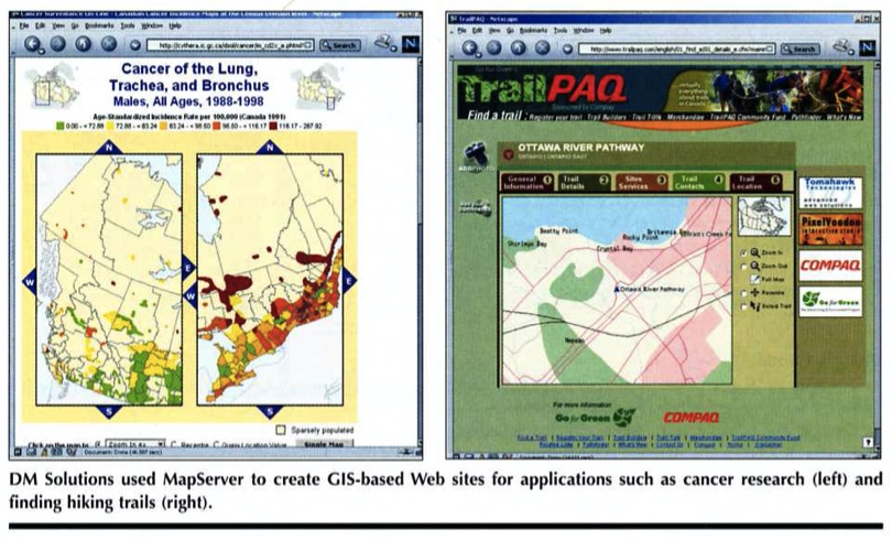
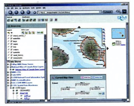
This article (PDF) was published in the August 2002 edition of GeoWorld. I came across my hard copy cleaning my desk and thought it might be of historical interest.
They say you can have your software good, cheap or soon, but you can’t have all three. Information technology (IT) project managers have assumed since the dawn of microchips that any improvement in one measure of software quality must inevitably be accompanied by a reduction in others.
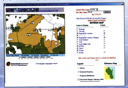
Last year, Ross Searle of the Department of Natural Resources and Mines, Queensland, Australia, faced this “three-horned” IT dilemma. He had a problem, and the solution had to be cheap, quick and good. Searle wanted to create an online permitting application that allowed resource officers in his department to quickly evaluate the environmental consequences of tree-clearing permits.
“In Queensland, our state government has legislation controlling the clearing of trees,” says Searle. “If a landholder wishes to clear trees, then he or she has to apply for a permit. A permit will only be issued if the clearing does not cause environmental degradation. The state government has the role of assessing the permits. To do this, officers need access to a broad range of clatasets all generally held in GIS form.”
The three-horned dilemma loomed. The application had to be cheap—budgets for the department were shrinking, no discretionary funding was available, and all the existing licenses for proprietary Web mapping software were tied up in the departmental head office. The application had to be good—data volumes were huge, encompassing several spatial coverages of more than 500MB apiece, so lightweight solutions weren’t going to work. The application had to be ready soon—Searle didn’t have the time or money to program a complex system from scratch.
Searle slew his three-homed dilemma with a combination of “open-source” tools, using the University of Minnesota (LIMN) MapServer to provide Web mapping capabilities and PostGIS/PostgreSQL as the spatial database backend.
“We are using PostGIS to deliver large amounts of natural resource information via a MapServer interface,” adds Searle, “The MapServer/PostGIS application allows users to quickly search for a parcel of land and bring up all the relevant information in a standard format.
“Apart from the cost factors, I believe that the open-source software for this particular purpose is every bit as good—if not better—than the solutions offered by commercial vendors. We have found that the developers of open-source software are responsive to bugs/suggestions/inquiries, etc., more than commercial vendors. In fact, one of the biggest problems we have found in using open source is keeping up with all the improvements.”
What’s Open Source?
Unlike “freeware” or “shareware,” open-source software provides users with more than just a program and some documentation. As defined by the Open Source Initiative, open-source software “must be distributed under a license that guarantees the right to read, redistribute, modify and use the software freely.”
Open-source programs are distributed along with their “source code,” i.e., the programming instructions that control how the software works. Using open-source software is like eating at a restaurant where the recipes are served alongside the meals—you can simply enjoy the food, but you also have the option of taking the recipe home, changing the seasonings and serving the result to your friends.
Successful open-source projects attract developers interested in improving the software. Sometimes their motives are personal, but often they’re professional—the software helps solve a problem, and improvements to the software make doing their job easier. Through time, success breeds success. The projects with the most development activity attract more developers and become more active, improving and addling features at a rapid rate.
After users become accustomed to having complete access to the inner workings of the software they use, proprietary software begins to feel a little limiting, even unnatural. Bob Young, co-founder of the successful open-source company Red Hat, likes to compare purchasing proprietary software to “buying a car with the hood welded shut.”
“We demand the ability to open the hood of our cars, because it gives us, the consumer, control over the product we’ve bought and takes it away from the vendor,” notes Young.
In Young’s view, the software market should be one in which consumers don’t purchase software per se, but instead purchase whatever services they need to effectively use the software they choose.
Rather than purchase a proprietary database system and then purchase support from the proprietary database company, customers instead choose an open-source database and purchase support from an array of support companies with expertise in the chosen database. The net effect is the same—customers have functioning and supported products—but the balance of power is shifted in favor of customers.
An Open-Source Economy
In a healthy open-source economy, every successful open-source software project should have an accompanying set of companies prepared to offer support and consulting to customers who choose to implement systems with the software. DM Solutions Group, for example, is one of the companies supporting the LIMN MapServer—the open-source Web mapping application Searle used to implement his online permitting application. DM Solutions started as a traditional systems integrator, providing consulting services that implement proprietary software packages.
“We were frustrated with the fact that we were dealing with ‘closed boxes’ that magically did all the work for us,” says Dave Mcllhagga, president of DM Solutions, “If it didn’t do it the way we wanted it to, we couldn’t change it or would have to depend and wait on a third party to take care of any problems.
“Now that we are using open-source software, we’re in full control of the situation and can offer not only consulting services, but also free and open software to base it on. We then can guarantee that if there are any problems in the base software, we can fix them. The word ‘workaround’ no longer is part of our vocabulary. If it doesn’t work, we fix it.”
In addition to providing MapServer consulting services, DM Solutions soon became actively involved in MapServer development, adding new features like OpenGIS Web Map Server, Macromedia Flash and GML support. Mcllhagga notes that effort spent on development actually promotes consulting skills, demonstrating that “we are the industry leaders in use of the product, have a high level of expertise and can therefore offer a premium service to our clients.”
Refractions Research occupies a similar position with respect to PostGIS/PostgreSQL, Searle’s other key application component. As the original developers and current maintainers of PostGIS, Refractions Research occupies a market niche and can offer special expertise to the growing community of PostGIS users. Dave Blasby, principal developer of PostGIS, wonders where it’s all leading.
“If you had told me last year that we would be working for clients in Germany, Florida, Montreal and Los Angeles during the next 12 months, I would have thought you were crazy,” says Blasby.
An Unlocked Hood
Products like UMN MapServer and PostGIS/PostgreSQL gain leverage by building on the prior efforts of other open-source projects. For example, by building on the capabilities of PostgreSQL, PostGIS gains all the strengths of an existing industrial-strength database: transactional integrity, write-ahead logs, Structured Query Language (SQL) and standard application programming interfaces.
Similarly, MapServer garners much of its GIS file format compatibility by using OGR and Geospatial Data Abstraction Library (GDAL) file format libraries. Shared code such as software libraries is extremely important to open-source projects, because it allows all projects to improve together in lockstep as enhancements are made to base libraries.
The author of the OGR and GDAL libraries is Frank Warmerdam, an independent contractor in Ontario, Canada. Warmerdam provides customizations of his many geospatial libraries to software companies and system integrators, who bundle the libraries in their products.
“In many cases, the clients gain substantial leverage from building on an existing open-source library, only needing to pay for the specific improvements they require,” explains Warmerdam. “Clients funding initial work on libraries often gain from testing and improvements provided by later users.”
Ironically, Warmerdam’s open-source TIFF image-format library is the basis for TIFF support in several well-known proprietary GIS products as well as many open-source projects. Even proprietary software vendors can take advantage of the group source libraries provide.
Warmerdam has been working in the software industry for many years and says one of the reasons he now works mainly on open-source contracts “is the sense that I’m building something that will outlast the commercial decisions and market success of any one company.”
Future Solutions
As the foundation of several open-source projects, Warmerdam’s libraries will be used for many years. The sheer quantity of open-source GIS projects available can be appreciated by browsing the entries at FreeGIS.org, a clearinghouse Web site for project information.
Unlike Linus Torvalds, the author of Linux, open-source GIS promoters don’t talk of “world domination”—not even in jest as Torvalds did. Instead, they point to the flexibility that’s the hallmark of open-source software and predict increasing ubiquity behind the scenes.
Dave Mcllhagga points to MapServer as an example of open-source GIS infrastructure with strong momentum, and notes the importance of providing a viable alternative to the status quo.
“There’s a reason why MapServer’s user base has been growing,” notes Mcllhagga. “With the availability of user-friendly tools complementing some technically robust technology, there’s reason to believe it can play a substantial role in this business. If open-source alternatives can continue to improve and at least keep commercial vendors honest, they will be successful.”
Regardless of whether open-source OS ever lands on desktops and workstations, it likely will play an increasing role in meeting the specialized needs of the OS community. Wherever people have problems to solve and a willingness to share their solutions with others, open source will continue to flourish.
17 Oct 2021
Public accounts came out at the end of summer, so I have finally gotten around to entering in the central government data (the Health Authorities put out their reports much later) and the results show … the first decline since 2015?
Historically there have been growth pauses every 5 years or so, but the last two were associated with brief phases of government austerity, though that may have been a mirage, since the other thing the pauses all have in common is IBM taking it on the chin.
The loss of a book of Ministry of Health business (twice), then the loss of the desktop support contract, seem to tell the tale of IBM’s decline as an outsourcing juggernaut.
Maximus remains curiously resiliant, even as the MSP program phases out.
And the big shark, the back-office systems contract, which has migrated through a series of corporate names, from EDS (does anyone remember Ross Perot?) to HP Advanced Solutions to ESIT Advanced Solutions is now just … “Advanced Solutions, a DXC Technology Company”.

Looking over the sweep of the curve (which is now 23 years long!) you can see a bunch of interesting moments:
- The initial major privatization around 2005 under the Campbell Liberals, which starts off the whole process.
- The entry of Maximus into the Ministry of Health in 2005 at that same time, which may help explain some of the decline of IBM, as a more nimble competitor gobbles up prospects.
- The entry of Deloitte in 2011, for the Social Services ICM project, which leads to solid growth, but is also the high-water mark, as the planned successor project in Natural Resources around 2015 ends up going more to CGI than Deloitte.
What might the future hold? I have no idea, but unless and until the major backend contract held by “Advanced Solutions” changes (was supposed to run out this year?) I expect the total outsourcing spend to remain in the “holy cow that is a lot of money” range.

Coda: It’s waaaay to early to make any serious statements, but one thing I did notice eyeballing the vendors chart is that while most vendors have been treading water since the NDP took government in 2017, one “vendor” that has notched up 50% growth is my aggregate “local vendors” vendor, which I batch all the smaller companies into so they show up on the chart.
Since one of the NDP platform promises in 2017 was a preference to local companies, this could be sign of progress. Or it could be random! But local companies have gone from about $50M/yr to $75M/yr since 2017, that’s not nothing. Something to keep an eye on for next year.


