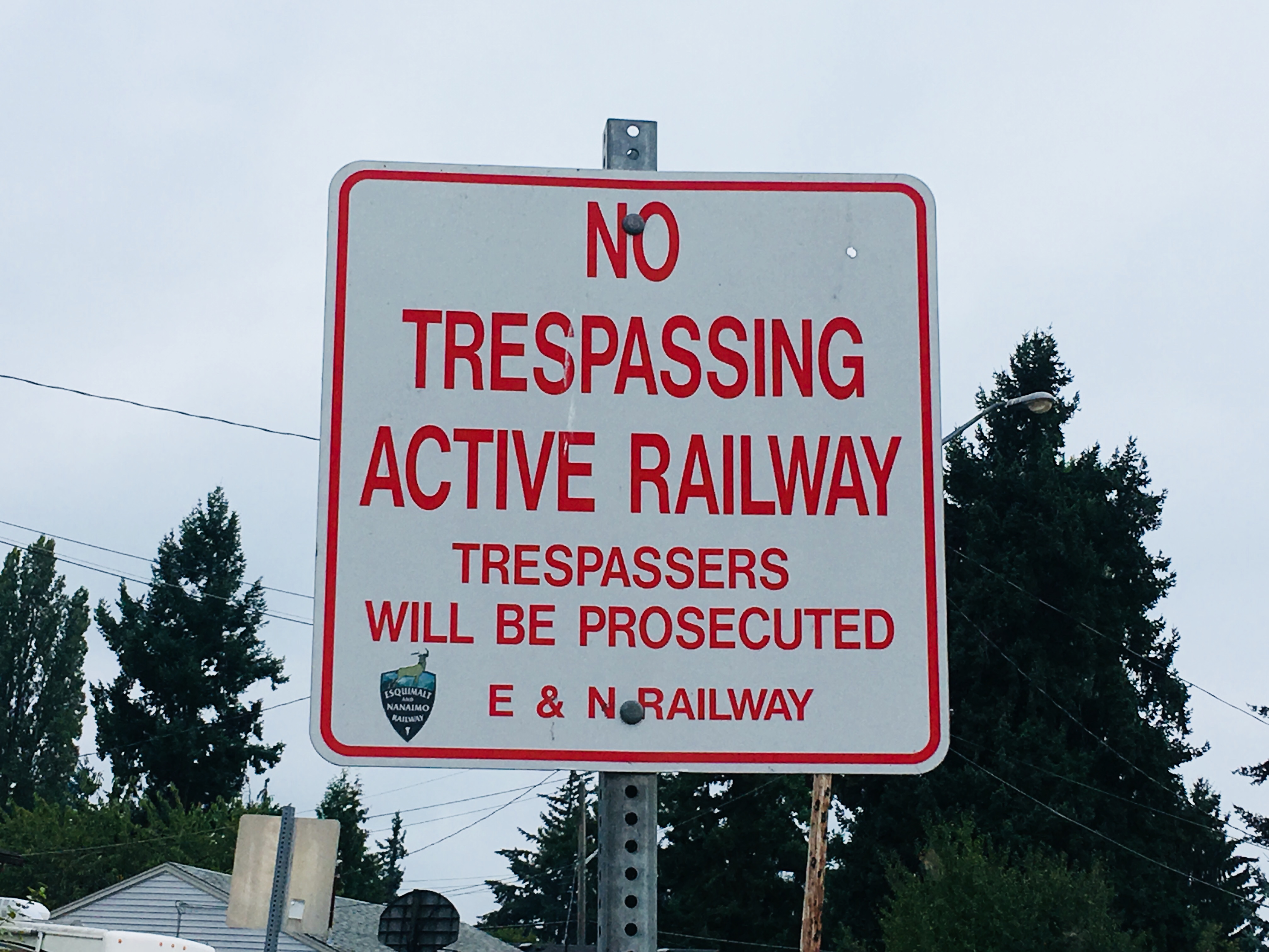
I also got to see a good portion of the old E&N railway line, as that line also passes through all the little towns I visited (with the exception of Cowichan Bay). It doesn’t take a trained surveyor to see that most of the railbed is in really poor condition. In many places the ties are rotting out, and you can pull spikes out of them with your bare hands. Running a train on the thing is going to take huge investments to basically rebuild the rail bed (and many of the trestles) from scratch, and the economics don’t work: revenues from freight and passenger service couldn’t even cover the operating costs of the line before it was shut down, let alone support a huge capital re-investment.
What to do with this invaluable right-of-way, an unobstructed ribbon of land running from Victoria to Courtenay (and beyond to Port Alberni)?
Unlike the current ghost railway, a recreational trail would pay for itself almost immediately.
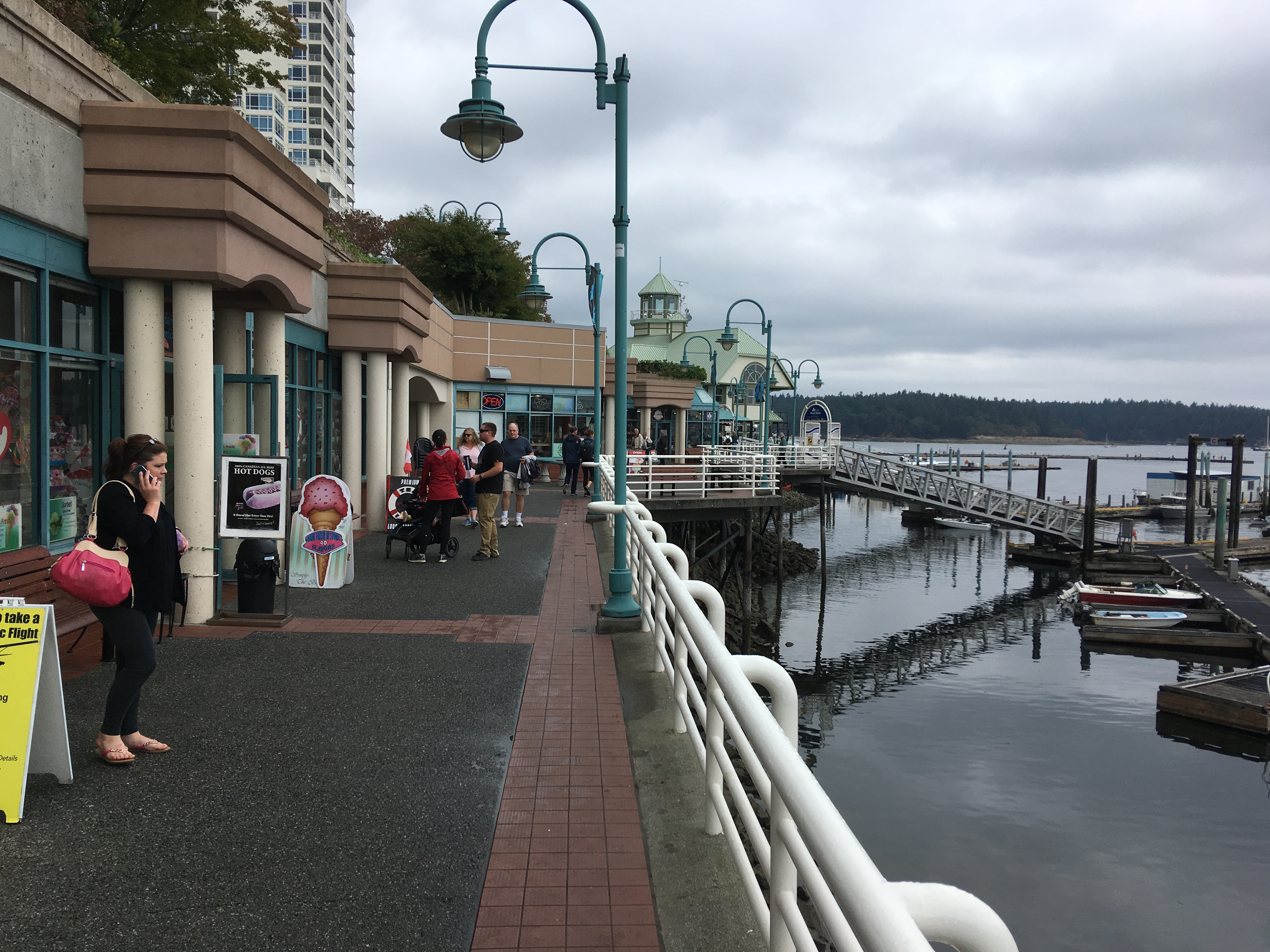
My first point of anecdata is my own 3-day bike excursion. Between accomodations, snacks along the way, and very tasty dinners (Maya Norte in Ladysmith and CView in Qualicum) I injected about $400 into the local economies over just two nights.
My second point of anecdata is an economic analysis of the Rum Runner’s Trail in Nova Scotia. The study shows annual expenditures by visitors alone of $3M per year. That doesn’t even count the economic benefit of local commuting and connection between communities.
My third point of anecdata is to just multiply $200 per night by three nights (decent speed) to cover the whole trail and 2000 marginal new tourists on the trail to get $1.2M direct new dollars. I find my made-up numbers are very compelling.
My fourth point of anecdata is the Mackenzie Interchange, currently under construction for over $70M. There is no direct economic benefit to this infrastructure, it will induce no tourist dollars and generate no long term employment.
If a Vancouver Island Rail Trail can generate even $3M in net new economic benefit for the province, it warrants a at least $50M investment to generate an ongoing 6% return. We spend more money for less return routinely (see the Mackenzie Interchange above).
And that’s just the tourism benefit.
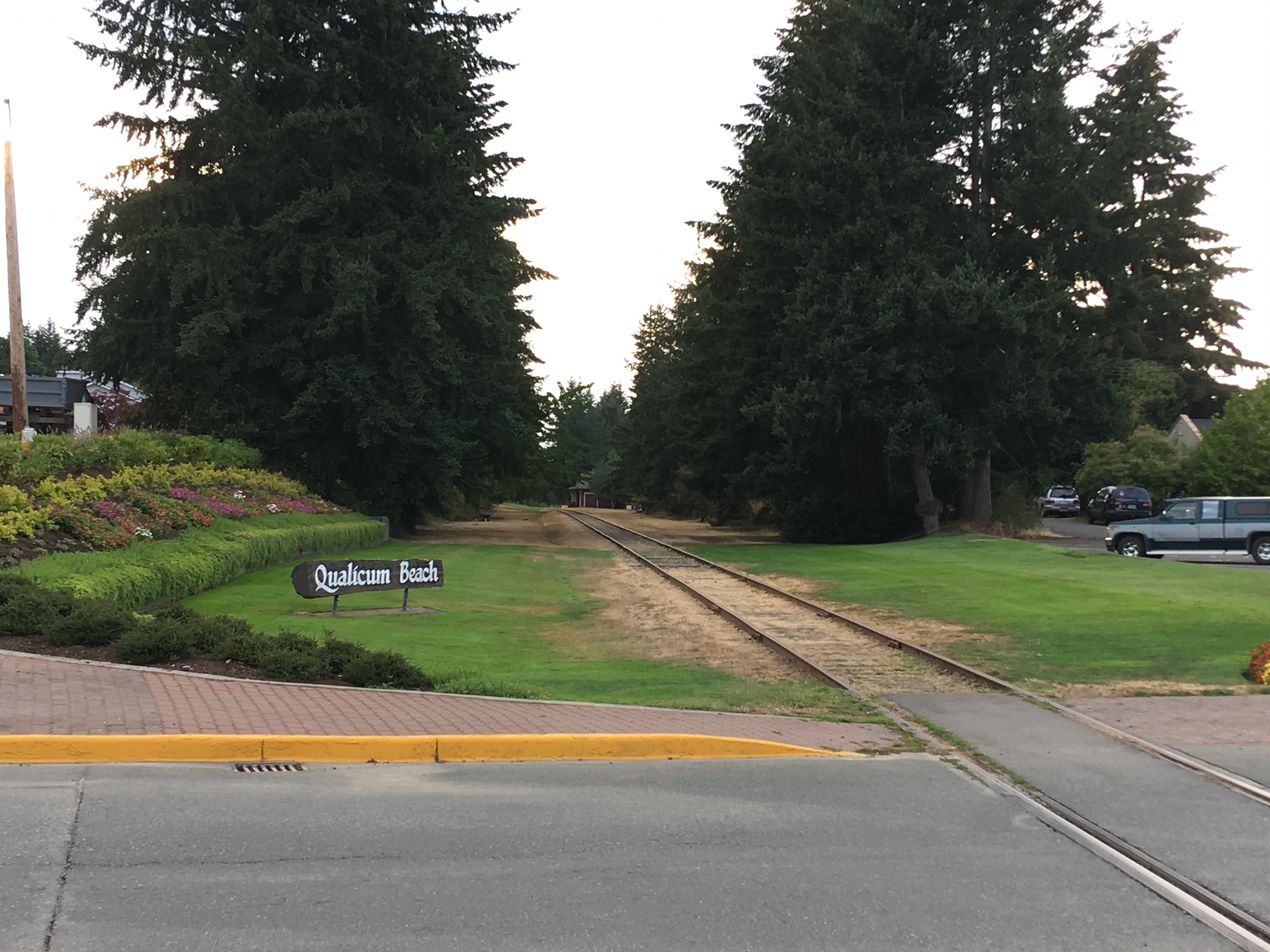
Electric bikes are coming, and coming fast. A paved, continuous trail will provide another transportation alternative that is currently unavailable. Take it from me, I rode from Nanaimo to Parksville on the roaring busy highway 19 through Nanoose: it’s a terrible experience, nobody wants to do that. Cruising a paved rail trail on a quietly whirring electic bike though, that would be something else again.
Right now the E&N line is not a transportation alternative. Nor is it a tourist destination. Nor is it a railway. It’s time to put that land back to work.
The results were less than stellar for my example data, which was small-but-not-too-small: under default settings of PostgreSQL and PostGIS, parallel behaviour did not occur.
However, unlike in previous years, as of PostgreSQL 10, it was possible to get parallel plans by making changes to PostGIS settings only. This was a big improvement from PostgreSQL 9.6, which substantial changes to the PostgreSQL default settings were needed to force parallel plans.
PostgreSQL 11 promises more improvements to parallel query:
Parallelized hash joins
Parallelized CREATE INDEX for B-tree indexes
Parallelized CREATE TABLE .. AS, CREATE MATERIALIZED VIEW, and certain queries using UNION
With the exception of CREATE TABLE ... AS none of these are going to affect spatial parallel query. However, there have also been some none-headline changes that have improved parallel planning and thus spatial queries.
TL;DR:
PostgreSQL 11 has slightly improved parallel spatial query:
Costly spatial functions on the query target list (aka, the SELECT ... line) will now trigger a parallel plan.
Under default PostGIS costings, parallel plans do not kick in as soon as they should.
Parallel aggregates parallelize readily under default settings.
Parallel spatial joins require higher costings on functions than they probably should, but will kick in if the costings are high enough.
Setup
In order to run these tests yourself, you will need:
PostgreSQL 11
PostGIS 2.5
You’ll also need a multi-core computer to see actual performance changes. I used a 4-core desktop for my tests, so I could expect 4x improvements at best.
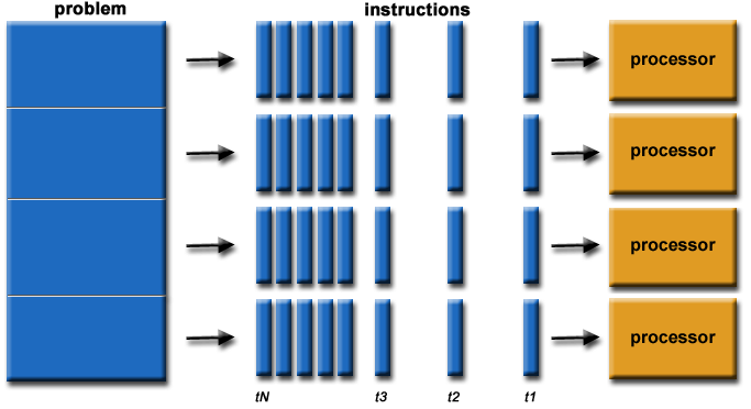
We will work with the default configuration parameters and just mess with the max_parallel_workers_per_gather at run-time to turn parallelism on and off for comparison purposes.
When max_parallel_workers_per_gather is set to 0, parallel plans are not an option.
max_parallel_workers_per_gather sets the maximum number of workers that can be started by a single Gather or Gather Merge node. Setting this value to 0 disables parallel query execution. Default 2.
Before running tests, make sure you have a handle on what your parameters are set to: I frequently found I accidentally tested with max_parallel_workers set to 1, which will result in two processes working: the leader process (which does real work when it is not coordinating) and one worker.
Boom! Parallel scan with three workers. This is an improvement from PostgreSQL 10, where a spatial function on the target list would not trigger a parallel plan at any cost.
Joins
Starting with a simple join of all the polygons to the 100 points-per-polygon table, we get:
In order to give the PostgreSQL planner a fair chance, I started with the largest table, thinking that the planner would recognize that a “70K rows against 7M rows” join could use some parallel love, but no dice:
Nested Loop
(cost=0.41..13555950.61 rows=1718613817 width=2594)
 ->  Seq Scan on pd
     (cost=0.00..14271.34 rows=69534 width=2554)
 ->  Index Scan using pts_gix on pts
     (cost=0.41..192.43 rows=232 width=40)
       Index Cond: (pd.geom && geom)
       Filter: _st_intersects(pd.geom, geom)
As with all parallel plans, it is a nested loop, but that’s fine since all PostGIS joins are nested loops.
First, note that our query can be re-written like this, to expose the components of the spatial join:
So for operator-only queries, it seems the only way to force a spatial join is to muck with the parallel_tuple_cost parameter.
Costing PostGIS?
A relatively simple way to push more parallel behaviour out to the PostGIS user community would be applying a global increase of PostGIS function costs. Unfortunately, doing so has knock-on effects that will break other use cases badly.
In brief, PostGIS uses wrapper functions, like ST_Intersects() to hide the index operators that speed up queries. So a query that looks like this:
SELECT...FROM...WHEREST_Intersects(A,B)
Will be expanded by PostgreSQL “inlining” to look like this:
SELECT...FROM...WHEREA&&BAND_ST_Intersects(A,B)
The expanded version includes both an index operator (for a fast, loose evaluation of the filter) and an exact operator (for an expensive and correct evaluation of the filter).
If the arguments “A” and “B” are both geometry, this will always work fine. But if one of the arguments is a highly costed function, then PostgreSQL will no longer inline the function. The index operator will then be hidden from the planner, and index scans will not come into play. PostGIS performance falls apart.
It is possible to change current inlining behaviour with a very small patch but the current inlining behaviour is useful for people who want to use SQL wrapper functions as a means of caching expensive calculations. So “fixing” the behaviour PostGIS would break it for some non-empty set of existing PostgreSQL users.
Tom Lane and Adreas Freund briefly discussed a solution involving a smarter approach to inlining that would preserve both the ability inline while avoiding doing double work when inlining expensive functions, but discussion petered out after that.
As it stands, PostGIS functions cannot be properly costed to take maximum advantage of parallelism until PostgreSQL inlining behaviour is made more tolerant of costly parameters.
Conclusions
PostgreSQL seems to weight declared cost of functions relatively low in the priority of factors that might trigger parallel behaviour.
In sequential scans, costs of 100+ are required.
In joins, costs of 10000+ are required. This is suspicious (100x more than scan costs?) and even with fixes in function costing, probably not desireable.
Required changes in PostGIS costs for improved parallelism will break other aspects of PostGIS behaviour until changes are made to PostgreSQL inlining behaviour…
Today is my first day with my new employer Crunchy Data. Haven’t heard of them? I’m not surprised: outside of the world of PostgreSQL, they are not particularly well known, yet.
I’m leaving behind a pretty awesome gig at CARTO, and some fabulous co-workers. Why do such a thing?
While CARTO is turning in constant growth and finding good traction with some core spatial intelligence use cases, the path to success is leading them into solving problems of increasing specificity. Logistics optimization, siting, market evaluation.
Moving to Crunchy Data means transitioning from being the database guy (boring!) in a geospatial intelligence company, to being the geospatial guy (super cool!) in a database company. Without changing anything about myself, I get to be the most interesting guy in the room! What could be better than that?
Crunchy Data has quietly assembled an exceptionally deep team of PostgreSQL community members: Tom Lane, Stephen Frost, Joe Conway, Peter Geoghegan, Dave Cramer, David Steele, and Jonathan Katz are all names that will be familiar to followers of the PostgreSQL mailing lists.
They’ve also quietly assembled expertise in key areas of interest to large enterprises: security deployment details (STIGs, RLS, Common Criteria); Kubernetes and PaaS deployments; and now (ta da!) geospatial.
Why does this matter? Because the database world is at a technological inflection point.
Core enterprise systems change very infrequently, and only under pressure from multiple sources. The last major inflection point was around the early 2000s, when the fleet of enterprise proprietary UNIX systems came under pressure from multiple sources:
The RISC architecture began to fall noticeably behind x86 and particular x86-64.
Pricing on RISC systems began to diverge sharply from x86 systems.
A compatible UNIX operating system (Linux) was available on the alternative architecture.
A credible support company (Red Hat) was available and speaking the language of the enterprise.
The timeline of the Linux tidal wave was (extremely roughly):
90s - Linux becomes the choice of the tech cognoscenti.
00s - Linux becomes the choice of everyone for greenfield applications.
10s - Linux becomes the choice of everyone for all things.
By my reckoning, PostgreSQL is on the verge of a Linux-like tidal wave that washes away much of the enterprise proprietary database market (aka Oracle DBMS). Bear in mind, these things pan out over 30 year timelines, but:
Oracle DBMS offers no important feature differentiation for most workloads.
Oracle DBMS price hikes are driving customers to distraction.
Server-in-a-cold-room architectures are being replaced with the cloud.
PostgreSQL in the cloud, deployed as PaaS or otherwise, is mature.
A credible support industry (including Crunchy Data) is at hand to support migrators.
I’d say we’re about half way through the evolution of PostgreSQL from “that cool database” to “the database”, but the next decade of change is going to be the one people notice. People didn’t notice Linux until it was already running practically everything, from web servers to airplane seatback entertainment systems. The same thing will obtain in database land; people won’t recognize the inevitability of PostgreSQL as the “default database” until the game is long over.
Having a chance to be a part of that change, and to promote geospatial as a key technology while it happens, is exciting to me, so I’m looking forward to my new role at Crunchy Data a great deal!
Meanwhile, I’m going to be staying on as a strategic advisor to CARTO on geospatial and database affairs, so I get to have a front seat on their continued growth too. Thanks to CARTO for three great years, I enjoyed them immensely!
A year has gone by and the public accounts are out again, so I have updated my running tally of IT outsourcing for the BC government.
While the overall growth is modest, I’m less sure of my numbers this year because of last year’s odd and sudden drop-off of the IBM amount.
I am guessing that the IBM drop should be associated with their loss of desktop support services for the health authorities, which went to Fujitsu, but for some reason the transfer is not reflected in the General Revenue accounts. The likely reason is that it’s now being paid out of some other bucket, like the Provincial Health Services Authority (PHSA), so fixing the trend line will involve finding that spend in other accounts. Unfortunately, Health Authorities won’t release their detailed accounts for another few months.
All this shows the difficulty in tracking IT spend over the whole of government, which is something the Auditor General remarked on when she reviewed IT spending a few years ago. Capital dollars are relatively easy to track, but operating dollars are not, and of course the spend is spread out over multiple authorities as well as in general revenue.
In terms of vendors, the drop off in HP/ESIT is interesting. For those following at home ESIT (formerly known as HP Advanced Solutions) holds the “back-office” contract, which means running the two government data centres (in Calgary and Kamloops (yes, the primary BC data centre is in Alberta)) as well as all the servers therein and the networks connecting them up. It’s a pretty critical contract, and the largest in government. Since being let (originally to Ross Perot’s EDS), one of the constants of this tracking has been that the amount always goes up. So this reduction is an interesting data point: will it hold?
And there’s still a large whale unaccounted for: the Coastal Health Authority electronic health record project, which has more-or-less dropped off the radar since Adrian Dix brought in Wynne Powell as a fixer. The vendors (probably Cerner and others) for that project appear on neither the PHSA nor Coastal Health public accounts, I think because it is all being run underneath a separate entity. I haven’t had a chance to figure out the name of it (if you know the way this is financed, drop me a line).
One of the joys of geospatial processing is the variety of tools in the tool box, and the ways that putting them together can yield surprising results. I have been in the guts of PostGIS for so long that I tend to think in terms of primitives: either there’s a function that does what you want or there isn’t. I’m too quick to ignore the power of combining the parts that we already have.
A community member on the users list asked (paraphrased): “is there a way to split a polygon into sub-polygons of more-or-less equal areas?”
I didn’t see the question, which is lucky, because I would have said: “No, you’re SOL, we don’t have a good way to solve that problem.” (An exact algorithm showed up in the Twitter thread about this solution, and maybe I should implement that.)
PostGIS developer Darafei Praliaskouskidid answer, and provided a working solution that is absolutely brilliant in combining the parts of the PostGIS toolkit to solve a pretty tricky problem. He said:
The way I see it, for any kind of polygon:
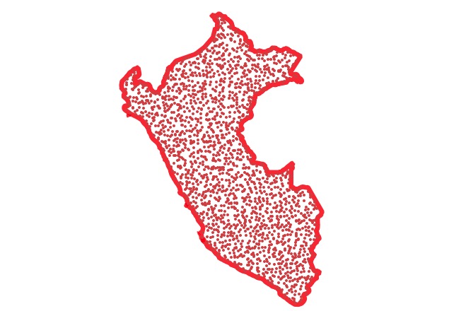
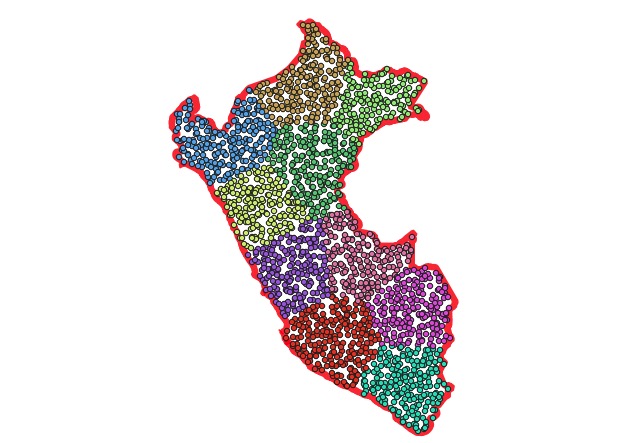
Convert a polygon to a set of points proportional to the area by ST_GeneratePoints (the more points, the more beautiful it will be, guess 1000 is ok);
Decide how many parts you’d like to split into, (ST_Area(geom)/max_area), let it be K;
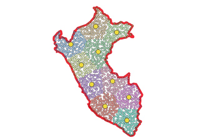
Take KMeans of the point cloud with K clusters;
For each cluster, take a ST_Centroid(ST_Collect(point));
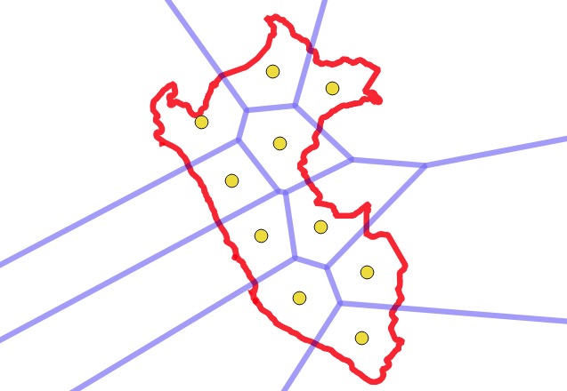
Feed these centroids into ST_VoronoiPolygons, that will get you a mask for each part of polygon;
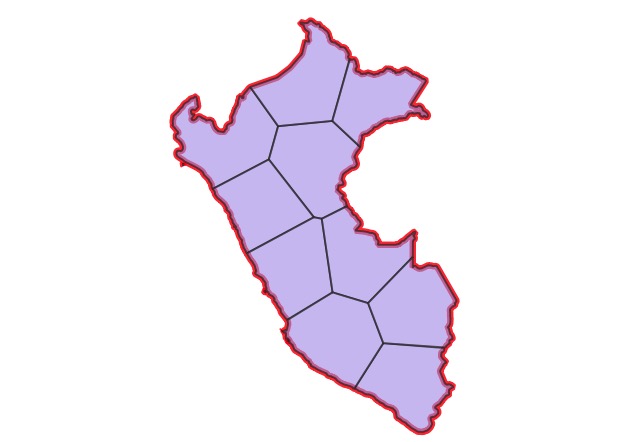
ST_Intersection of original polygon and each cell of Voronoi polygons will get you a good split of your polygon into K parts.
Let’s take it one step at a time to see how it works.
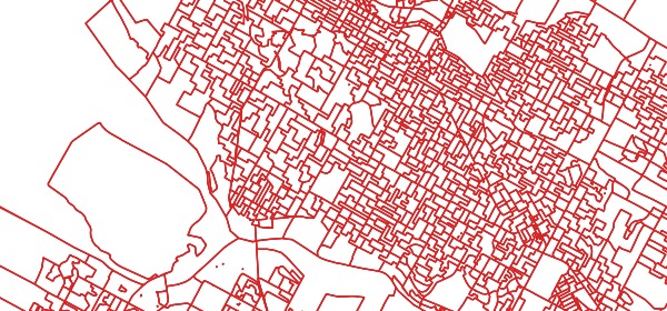
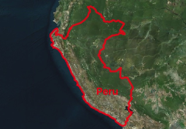
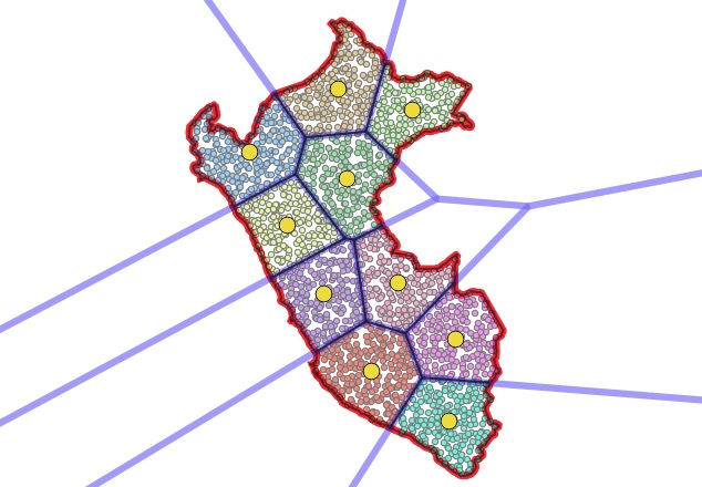
We’ll use Peru as the example polygon, it’s got a nice concavity to it which makes it a little trickier than an average shape.
Now, cluster the point field, setting the number of clusters to the number of pieces you want the polygon divided into. Visually, you can now see the divisions in the polygon! But, we still need to get actual lines to represent those divisions.
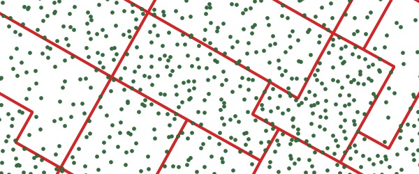
Now, use a voronoi diagram to get actual dividing edges between the cluster centroids, which end up closely matching the places where the clusters divide!
Finally, intersect the voronoi areas with the original polygon to get final output polygons that incorporate both the outer edges of the polgyon and the voronoi dividing lines.
Clustering a point field to get mostly equal areas, and then using the voronoi to extract actual dividing lines are wonderful insights into spatial processing. The final picture of all the components of the calculation is also beautiful.
I’m not 100% sure, but it might be possible to use Darafei’s technique for even more interesting subdivisions, like “map of the USA subdivided into areas of equal GDP”, or “map of New York subdivided into areas of equal population” by generating the initial point field using an economic or demographic weighting.