17 May 2023
Last month I got to record a couple podcast episodes with the MapScaping Podcast’s Daniel O’Donohue. One of them was on the benefits and many pitfalls of putting rasters into a relational database, and it is online now!
TL;DR: most people think “put it in a database” is a magic recipe for: faster performance, infinite scalability, and easy management.
Where the database is replacing a pile of CSV files, this is probably true.
Where the database is replacing a collection of GeoTIFF imagery files, it is probably false. Raster in the database will be slower, will take up more space, and be very annoying to manage.
So why do it? Start with a default, “don’t!”, and then evaluate from there.
For some non-visual raster data, and use cases that involve enriching vectors from raster sources, having the raster co-located with the vectors in the database can make working with it more convenient. It will still be slower than direct access, and it will still be painful to manage, but it allows use of SQL as a query language, which can give you a lot more flexibility to explore the solution space than a purpose built data access script might.
There’s some other interesting tweaks around storing the actual raster data outside the database and querying it from within, that I think are the future of “raster in (not really in) the database”, listen to the episode to learn more!
09 May 2023
I can only imagine how much AI large language model generated junk there is on the internet already, but I have now personally found one in my blog comments. It’s worth pointing out, since comment link spam is a long time scourge of web publishing, and the new technology makes it just that little extra bit invisible.
The target blog post is this one from the late 2000’s oil price spike. A brief post about how transportation costs tie into real estate desirability. (Possible modern day tie in: will the rise of EVs and decoupling of daily transport costs from oil prices result in a suburban rennaisance? God I hope not.)
The LLM spam by “Liam Hawkins” is elegant in its simplicity.

I imagine the prompt is nothing more complex than “download this page and generate 20 words that are a reasonable comment on it”. The link goes to a Brisbane bathroom renovation company, that I am sure does sterling work and maybe should concentrate on word of mouth rather than SEO.
I need to check my comment settings, since the simplest solution is surely to just disallow links in comments. An unfortunate degredation in the whole point of the “web”, but apparently necessary in these troubled times.
30 Apr 2023
It is the age of the unbundled subscription, and I am wondering how long it will last? And also, what do our subscriptions say about us?
Here are mine in approximate order of acquisition:
- New Yorker Magazine, I have been a New Yorker subscriber for a very long time, and for a period in my life it was almost the only thing I read. I would read one cover-to-cover and by the time I had finished, the next would be in the mail box, and the cycle would repeat.
- Amazon Prime, I was 50/50 on this one until the video was added, and then I was fully hooked. It’s pricey, and intermittently has things I want to watch, so I often flirt with cancelling, but not so far.
- Netflix, for a while this was too cheap to not get, the kids liked some of it, I liked some, there were movies I enjoyed. However, the quality of is going down and the price up so it might be my first streamer cancellation.
- Washington Post, I got lucky and snagged a huge deal for international subscribers which has since disappeared, but got me a $2 / month subscription I couldn’t say “no” to, because I do read a lot of WP content.
- Talking Points Memo, the best independent political journalism site, which was pivoting to subscription years before it became cool. My first political read of every day.
- The New York Times, a very pricey pleasure, but I found myself consuming a lot of NYT content, and finally felt I just had to buck up.
- Disney+, for my son who was dying to see all the Star Wars and Marvel content. Now that he’s watched it all, we are discovering some of their other offerings, they own a quality catalogue.
- Spotify, once the kids were old enough to have smart phones, the demand for Spotify was pretty immediate. I’ve enjoyed having access to this huge pile of music too (BNL forever!).
- Slow Boring / Matt Yglesias, my first sub-stack subscription. You can tell a lot about my political valence from this.
- Volts / David Roberts, highly highly recommended if you are a climate policy nerd, as he covers climate and energy transition from every angle. Never easy, never simplistic, always worth the time.
In the pre-internet days I was also a subscriber to Harper’s and The Atlantic, but dropped both subscriptions some time ago. The articles in Harper’s weren’t grabbing me.
The real tragedy was The Atlantic, which would publish something I really wanted to read less than once a month, so I would end up … reading it on the internet for free. The incentive structure for internet content is pretty relentless in terms of requiring new material very very frequently, and a monthly publication like The Atlantic fits that model quite poorly.
Except for Volts, this list of paid subscriptions is curiously devoid of a huge category of my media consumption: podcasts. I listen to Ezra Klein, Chris Hayes, Strict Scrutiny, Mike Duncan, and Odd Lots for hours a week, for free. This feels… off kilter.
Although I guess a some of these podcasts are brand embassadors for larger organizations (NYT, NBC, Bloomberg), it seems hard to believe advertising is really the best model, particularly for someone like Mike Duncan who has established a pretty big following.
(If Mike Duncan committed to another multi-year history project, I’d sign up!)
One thing I haven’t done yet is tot up all these pieces and see how they compare to my pre-internet subscription / media consumption bill. A weekend newspaper or two every week. Cable television. The three current affairs magazines. The weekly video rental. Even taken ala carte, I bet the old fashioned way of buying did add up over the course of a year.
I’m looking forward to a little more consolidation, particularly in the individual creator category. Someone will crack the “flexible bundle” problem to create the “virtual news magazine” eventually, and I’m looking forward to that.
02 Feb 2023
Last week a user noted on the postgis-users list (paraphrase):
I upgraded from PostGIS 2.5 to 3.3 and now the results of my coordinate transforms are wrong. There is a vertical shift between the systems I’m using, but my vertical coordinates are unchanged.
Hmmm.
PostGIS gets all its coordinate reprojection smarts from the proj library. The user’s query looked like this:
SELECT ST_AsText(
    ST_Transform('SRID=7405;POINT(545068 258591 8.51)'::geometry,
    4979
    ));
“We just use proj” is a lot less certain and stable an assertion than it appears on the surface. In fact, PostGIS “just uses proj” for proj versions from 4.9 all the way up to 9.2, and there has been a lot of change to the proj library over that sweep of releases.
- The API radically changed around proj version 6, and that required a major rework of how PostGIS called the library.
- The way proj dereferenced spatial reference identifiers into reprojection algorithms changed around then too (it got much slower) which required more changes in how we interacted with the library.
- More recently the way proj handled “transformation grids” changed, which was the source of the complaint.
Exploring Proj
The first thing to do in debugging this “PostGIS problem” was to establish if it was in fact a PostGIS problem, or a problem in proj. There are commandline tools in proj to query what pipelines the system will use for a transform, and what the effect on coordinates will be, so I can take PostGIS right out of the picture.
We can run the query on the commandline:
echo 545068 258591 8.51 | cs2cs 'EPSG:7405' 'EPSG:4979'
Which returns:
52d12'23.241"N 0d7'17.603"E 8.510
So directly using proj we are seeing the same problem as in PostGIS SQL: no change in the vertical dimension, it goes in at 8.51 and comes out at 8.51. So the problem is not PostGIS, is is proj.
Cartographic transformations are nice deterministic functions, they take in a longitude and latitude and spit out an X and a Y.
(x,y) = f(theta, phi)
(theta, phi) = finv(x, y)
But not all transformations are cartographic transformations, some are transformation between geographic reference systems. And many of those are lumpy and kind of random.
For example, the North American 1927 Datum (NAD27) was built from classic survey techniques, starting from the “middle” (Kansas) and working outwards, chain by chain, sighting by sighting. The North American 1983 Datum (NAD83) was built with the assistance of the first GPS units. The accumulated errors of survey over distance are not deterministic, they are kind of lumpy and arbitrary. So the transformation from NAD27 to NAD83 is also kind of lumpy and arbitrary.
How do you represent lumpy and arbitrary transformations? With a grid! The grid says “if your observation falls in this cell, adjust it this much, in this direction”.
For the NAD27->NAD83 conversion, the NADCON grids have been around (and continuously improved) for a generation.
Here’s a picture of the horizontal deviations in the NADCON grid.
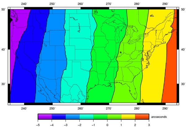
Transformations between vertical systems also frequently require a grid.
So what does this have to do with our bug? Well, the way proj gets its grids changed in version 7.
Grid History
Proj grids have always been a bit of an outlier. They are much larger than just the source code is. They are localized in interest (someone in New Zealand probably doesn’t need European grids), not everyone needs all the grids. So historically they were distributed in zip files separately from the code.
This is all well and good, but software packagers wanted to provide a good “works right at install” experience to their end users, so they bundled up the grids into the proj packages.
As more and more people consumed proj via packages and software installers, the fact that the grids were “separate” from proj became invisible to the end users: they just download software and it works.
This was fine while the collection of grids was a manageable size. But it is not manageable any more.
In working through the GDALBarn project to improve proj, Even Roualt decided to find all the grids that various agencies had released for various places. It turns out, there are a lot more grids than proj previously bundled. Gigabytes more.
Grid CDN
Simply distributing the whole collection of grids as a default with proj was not going to work anymore.
So for proj 7, Even proposed moving to a download-on-demand model for proj grids. If a transformation request requires a grid, proj will attempt to download the necessary grid from the internet, and save it in a local cache.
Now everyone can get the very best possible tranformation between system, everywhere on the globe, as long as they are connected to the internet.
Turn It On!
Except… the network grid feature is not turned on by default! So for versions of proj higher than 7, the software ships with no grids, and the software won’t check for grids on the network… until you turn on the feature!
There are three ways to turn it on, I’m going to focus on the PROJ_NETWORK environment variable because it’s easy to toggle. Let’s look at the proj transformation pipeline from our original bug.
projinfo -s EPSG:7405 -t EPSG:4979
The projinfo utility reads out all the possible transformation pipelines, in order of desirability (accuracy) and shows what each step is. Here’s the most desireable pipeline for our transform.
+proj=pipeline
  +step +inv +proj=tmerc +lat_0=49 +lon_0=-2 +k=0.9996012717 +x_0=400000
        +y_0=-100000 +ellps=airy
  +step +proj=hgridshift +grids=uk_os_OSTN15_NTv2_OSGBtoETRS.tif
  +step +proj=vgridshift +grids=uk_os_OSGM15_GB.tif +multiplier=1
  +step +proj=unitconvert +xy_in=rad +xy_out=deg
  +step +proj=axisswap +order=2,1
This transform actually uses two grids! A horizontal and a vertical shift. Let’s run the shift with the network explicitly turned off.
echo 545068 258591 8.51 | PROJ_NETWORK=OFF cs2cs 'EPSG:7405' 'EPSG:4979'

52d12'23.241"N  0d7'17.603"E 8.510
Same as before, and the elevation value is unchanged. Now run with PROJ_NETWORK=ON.
echo 545068 258591 8.51 | PROJ_NETWORK=ON cs2cs 'EPSG:7405' 'EPSG:4979'

52d12'23.288"N  0d7'17.705"E 54.462
Note that the horizontal and vertical results are different with the network, because we now have access to both grids, via the CDN.
No Internet?
If you have no internet, how do you do grid shifted transforms? Well, much like in the old days of proj, you have to manually grab the grids you need. Fortunately there is a utility for that now that makes it very easy: projsync.
You can just download all the files:
Or you can download a subset for your area of concern:
projsync --bbox 2,49,2,49
If you don’t want to turn on network access via the environment variable, you can hunt down the proj.ini file and flip the network = on variable.
22 Jan 2023
Last week, my friend and mentor Mark Sondheim died.
I am writing a little reluctantly, because I ever only knew a fraction of who Mark was. We were professional friends, we met and worked together because of technology and software. While I knew he was a devoted husband and father, I never really knew much of the texture or detail of those relationships, just that they were. So I cannot really celebrate Mark in full; perhaps it is the nature of modern life that it’s hard for anyone to be celebrated that way, but I do want to celebrate the person I knew.
I met Mark in 1997, early in my career, and was very fortunate to do so. By that point Mark was a manager in the BC government, overseeing a number of different projects in the mapping and analysis of resources, and one of those was a watershed analysis project I had managed to worm my way into as a sub-contractor.
It became very clear early on that Mark was interested in the details of what was going on in his projects. He wasn’t a “just get it done” manager, he was a “how is it going, what’s working what’s not, let’s talk about it” manager. He was endlessly curious and constructive, and that was something I tried to model later in my career when I had project teams of my own.
I think Mark’s curiousity manifested itself most in his willingness, his eagerness rather, to attack core problems in our field directly, rather than delegating the problems to a vendor or some other promise-maker. He trusted in the smart people around him, and I am proud to have been one of the smart people he trusted.
For most of you, Mark’s name will be one you haven’t heard before, but if you work in geospatial technology, you have been touched by his work, because it is woven all through the centre of the open source software you use.
I’ve mentioned this in talks in the past. Mark’s foresight in building the case and finding the funding for the development of JTS lead directly to GEOS which sits inside QGIS and PostGIS. And that was just one example of Mark’s willingness to take a risk to seed innovation in our industry.

Not all or even most of those seeds were open source. Safe Software (which makes our industry’s finest ETL tool, the FME) was born of Mark’s pursuit of a generic data standard, SAIF, that was used in BC for a couple decades. Mark contracted the founders of Safe to build the first SAIF translators and encouraged them to continue their work, which led to the FME and a still-flourishing local company.
Well before I met him, Mark led a team that built an early large scale analysis engine, CAPAMP, that was used for reporting and project work in BC for many years. Reading the acknowledgements Mark wrote, you can see him already working with teams of really smart people, building something detail oriented, not outsourcing risk and innovation, but gathering it close and nurturing it. I think it’s no coincidence that the list of collaborators also includes many of the future leaders of the BC geospatial sector.
I often tried to get Mark to admit the extent of his influence and importance to our industry, but he demurred. He’d point to his own professional models, like his early boss Art Benson, who granted him the freedom to experiment and explore within a government structure that too often defaulted to risk management and timidity. He paid forward his lessons though, and gave that same freedom to the people who worked for him, including me.
For me, that freedom meant being able to propose solutions that didn’t conform to “industry standards” as defined by government, but just worked. Superficially risky things like PostGIS and JTS and the FME that, 15 years after Mark was accepting and encouraging them, are now recognized as the workhorses of our industry.
The first production PostGIS database was run in our office and used as the backing store for another of Mark’s innovative projects, the BC Digital Road Atlas. Mark was PostGIS customer zero. Much of the early development of PostGIS was spurred by the needs of the DRA.
The BC Freshwater Atlas was built with PostGIS and JTS, after Mark turned around a project that was headed nowhere fast. In some ways, the project was a culmination of his earlier bets on PostGIS and JTS. The tools were at hand, because he’d incubated them years earlier. In the grand tradition of government, I don’t think Mark ever got credit for this project, which would have either not delivered, or delivered at 5x the cost if he hadn’t re-imagined it. Mostly he got grief, which he bore with gracious patience.
I don’t think I ever saw Mark get visibly angry. In fact, my first memory of him is an incident in which he was protecting me from the (loud, yelling) anger of his own boss, who felt (correctly, in all honestly) that I hadn’t moved a small project of his forward fast enough. Mark brought the temperature down, even though it was his own boss he was dealing with, and helped us focus on the work, what needed to get done. In the future, we dealt with no end of frustrating or potentially angering problems together, but his default was always calm, and always finding the next step to a solution.
In later years, when we had both left our connections with the provincial government behind, it was still always a pleasure to talk with Mark, because he retained his bottomless curiousity and willingness to honestly share. What was I working on, how was it hard, had I considered this approach? This is what he was thinking about, did I have any thoughts, should he do this? As an intellect, Mark was a friendly giant, he never calcified, and he didn’t arrive with a lot of ego. He was always a pleasure.
I will miss Mark a great deal, and our industry will too, even if mostly it doesn’t realize the debt it owes him. Thank you Mark, for all you shared with me on your journey.